Unraveling PaliGemma
A Peek at lightweight, open VLM along with deep dive in LLM internals.

Venturing into the Unknown
Coming from the medical domain and working especially with images, videos, and text modality, I've lately been intrigued by Visual-Language models. I started out trying to understand the whole field, but the industry has moved so fast over the last 3-4 years that just looking at the below contents overwhelmed me.
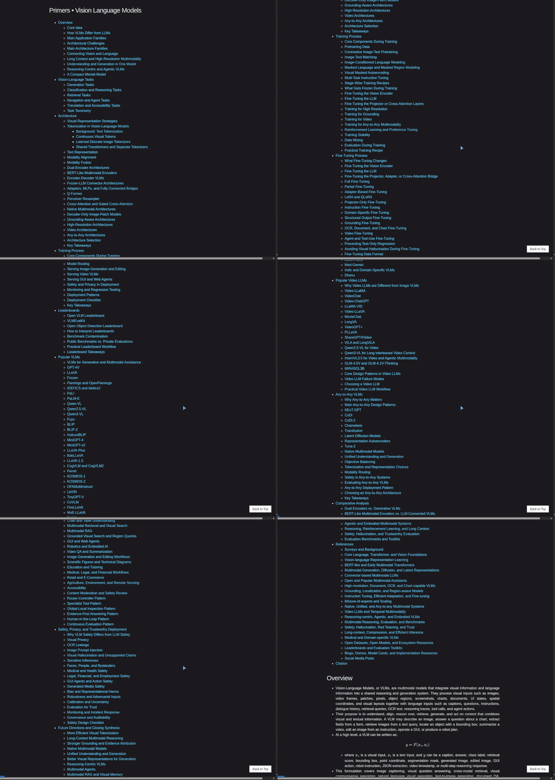
So instead, I picked one architecture to go deep on: PaliGemma. It's small, fully open with its weights and its detailed paper, made it easy for me to try it out locally. This is a long form blog covering not just Paligemma but also internals about attention mechanism, positional embeddings, layernorm(s), KV cache and many others.
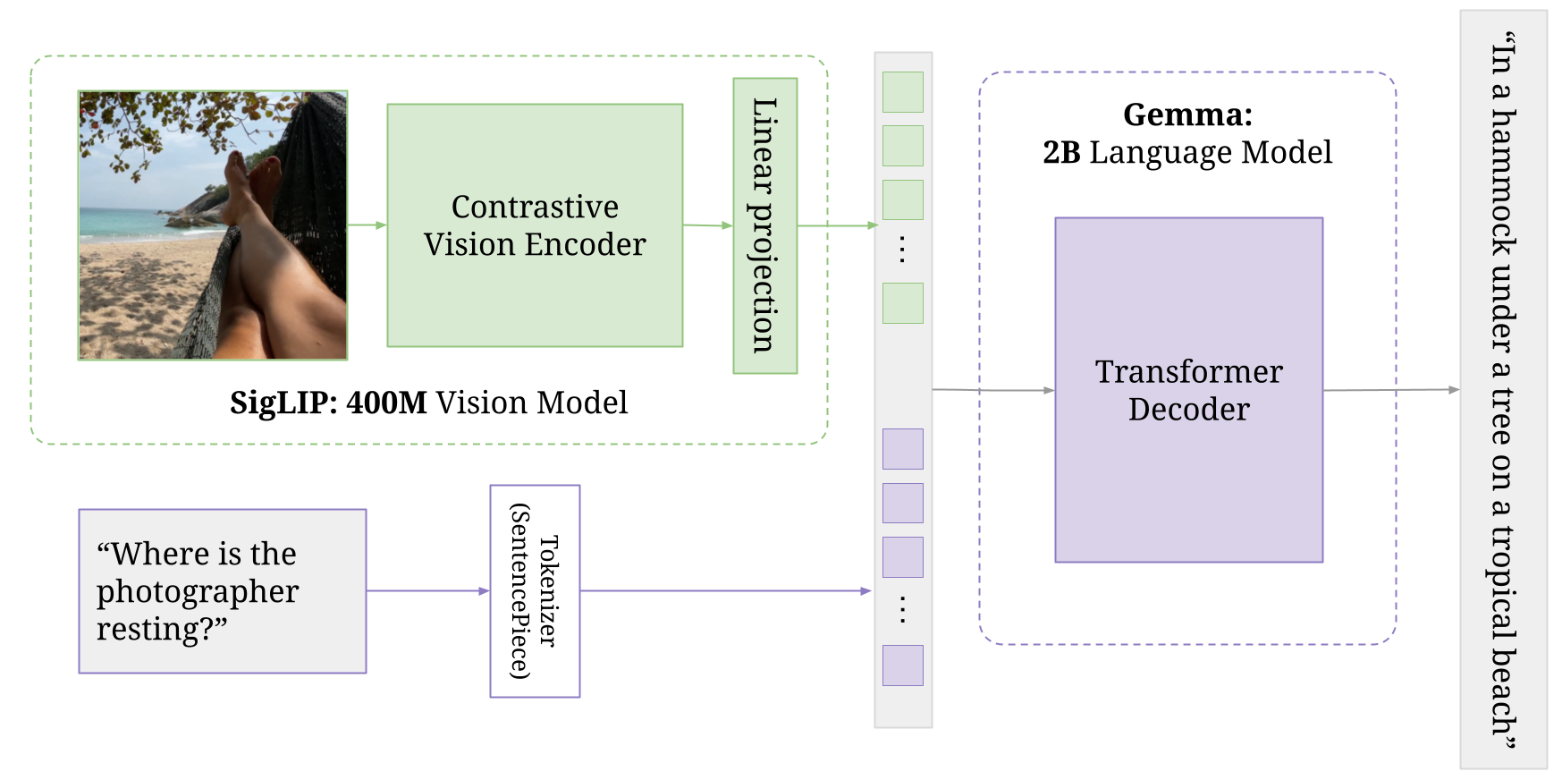
PaliGemma is a lightweight VLM (3 Billion Parameters in total) from Google. It utilizes open pretrained components like SigLIP image encoder and Gemma Language model.
It takes a image and a text as inputs and produces a text response token by token.
What all it can do
Before I start explaining the architecture, training recipe of the paligemma - let's look at what it offers. It's incredible how such a small vlm is capable of solving so many visual tasks like segmentation, object detection, image captioning , ocr - naming a few.
Image Captioning
PaliGemma can caption images when prompted to.

Visual Question Answering
PaliGemma can answer questions about an image, simply pass your question along with the image to do so.

Detection
PaliGemma can detect entities in an image using the detect [entity] prompt. It will output the location for the bounding box coordinates in the form of special <loc[value]> tokens, where value is a number that represents a normalized coordinate. Each detection outputs four location coordinates (y_min, x_min, y_max, x_max) followed by the detected label.

detect [entity] prompt.Referring Expression Segmentation
PaliGemma mix checkpoints can also segment entities in an image when given the segment [entity] prompt. This is called referring expression segmentation, because we refer to the entities of interest using natural language descriptions. The output combines location and segmentation tokens that can generate segmentation masks.

segment [entity] prompt. Source: huggingface.co/blog/paligemma.Document Understanding
PaliGemma mix checkpoints have great document understanding and reasoning capabilities.

PaliGemma Architecture
Paligemma utilizes Gemma's decoder only LLM architecture for its next token prediction capabilities. It uses a image encoder and projection layer to bring images into same token space to be supplied as a prompt to the gemma. For training the authors used a pretrained SigLIP 400M vision model as image encoder and a pretrained Gemma 2B Parameter as the LLM and then jointly trained these components on various visual-textual tasks.
SigLip
Before SigLip there was CLIP
CLIP, short for Contrastive Language-Image Pre-training, was released by OpenAI in 2021. It trains a joint embedding space for images and text from millions of image-caption pairs, entirely self-supervised, no manual labels involved. The idea is contrastive: pull a matching image-text pair's embeddings together, and push every other pair in the batch apart.
How CLIP Works
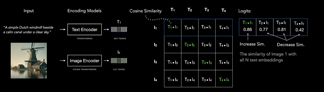
An image encoder and a text encoder turn a batch's images and texts into image and text embeddings. Every image embedding is dot-producted against every text embedding in the batch, after L2-normalizing both, producing a full image-by-text similarity matrix. The correct pairs sit on the diagonal, so the ground truth is just an identity matrix: image i should score high only against text j where i==j, and low against every other text in the batch.
Training this is a multiple-choice test repeated for every image: given all the texts in the batch, pick out the one that actually matches. Because each row is scored against every option at once. This is the first component of the loss. If you look closely it is a softmax function where you maximize the probability of the rightful dot product of image-text pair in that row.
Just like the images we will compute for text as well that will be using column wise softmax.

Problem with CLIP
All of the softmax functions in implementation are essentially "safe-softmax" in which you subtract the row maximum before exponentiation. This avoids the numerical stability issues which can happen with exponentials.
Formula 1.
In CLIP, the loss includes both text→image and image→text terms, which means two separate softmax computations: across images (columns) and across texts (rows). For numerical stability, you also need to scan max values twice (and often do two all-gathers). In other words, the softmax loss (or the image–text matrix shown below) is asymmetric, hard to parallelize, computationally expensive and harder to scale your batch across multiple GPUs.
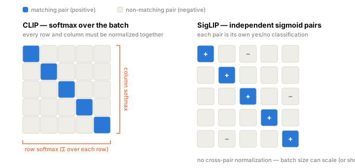
SigLIP reframes the CLIP's multiclass classification as a many binary classification tasks. CLIP taught image and text encoders to agree with each other by making every pair in a batch compete against every other pair. SigLIP asks a much smaller question of each pair, one at a time: is this image-text pair a match, yes or no?
SigLIP proposes replacing it with a sigmoid loss. Under this framing, each image–text pair's loss can be computed independently, without a global normalization factor. Each image–text dot product becomes an independent binary classification task.
With this optimization, you can scale batch size up to one million, and since computation is device-independent, it parallelizes nicely.
Why do we need pooling
As you will notice in the next section, the vision encoder returns (B, seq_len, dim) while SigLIP's contrastive loss operates on (B, dim). You can't dot-product a sequence against another sequence and get one similarity score per image, so you need a mechanism to pool (B, seq_len, dim) down to (B, dim). It can be done in two ways:
- CLS-token pooling (original CLIP): prepend a learnable
[CLS]token to the patch sequence; after the transformer, take only that token's output as the image embedding.
- Attention pooling (what SigLIP actually uses, a "MAP head", multihead attention pooling): a small learned query attends over all patch tokens and produces a single pooled vector. No CLS token needed.
SigLIP-So400m Vision Encoder
Pre Norm Vs Post Norm
Residual blocks were made popular by Resnets and have become a defacto for deeper stacked architectures. For a residual block $y = x + F(x)$. The gradient for x w.r.t Loss is:
The gradient is a sum, not a product: the upstream gradient passes straight through unchanged (the $I$ term), plus whatever correction the branch $F$ contributes.
Unroll over $L$ stacked blocks,
$x_l = x_{l-1}+F_l(x_{l-1})$,
so $x_L = x_0 + \sum_l F_l(x_{l-1})$
(here $x_l$ is the residual stream after block $l$, so $x_0$ is the input to the first block and $x_L$ is the final output after all $L$ blocks):
Compare this to a plain (non-residual) stack, $x_l = F_l(x_{l-1})$:
That's a product of $L$ Jacobians. Say each layer shrinks the gradient passing through it down to 90% of its size, a totally ordinary amount. After $L=27$ layers, which is SigLIP-So400m's actual depth, you get $0.9^{27}\approx 0.06$: only 6% of the gradient that reached the last layer makes it back to the first. Stack more layers and it decays exponentially toward zero, or explodes instead if each layer amplifies the gradient rather than shrinking it.
With the residual sum, there is no such product: $\partial L/\partial x_0$ always contains at least $\partial L/\partial x_L$ through the identity term, no matter how degenerate every individual $\partial F_l/\partial x_{l-1}$ gets. That additive identity term is the actual mechanism behind "residual connections fix vanishing gradients."
Pre-norm puts LayerNorm inside $F(x)$. Because LayerNorm only appears inside the branch, it never touches the raw identity term above, so a healthy, undiminished gradient signal reaches all the way from the last layer back to the first:
Here $I$ is a pure, unmodified identity. $J_{LN}$ only multiplies the branch term, it never wraps the whole expression. Unrolled, the skip path is the same clean additive sum as above, with no product of LayerNorm Jacobians ever touching the direct gradient highway.
Post-norm applies LayerNorm after $x+F(x)$, wrapping the whole sum, and this is what reduces gradient flow from the last layer back to the first:
The identity term $I$ is now multiplied by $J_{LN}$, no longer a clean pass-through. Unrolled over $L$ layers:
The characteristics of the $J_{LN,l}$ element in the above equation in simpler terms is, it carries a $1/\sigma$ rescaling (where $\sigma$ is that layer's per-token standard deviation from its own LayerNorm) and it is not full rank, since it collapses two directions to zero. So it is never exactly the identity.
But what about activations
We saw how pre-norm helps the backward pass through its additive identity-gradient property. But what about the actual $x$ values flowing forward, from the input to the last layer? Since $x_l = x_{l-1} + F_l(\operatorname{LN}(x_{l-1}))$, the main path itself is never normalized: every residual branch only adds more onto it, and nothing on that path ever rescales it back down. So $\|x\|$ keeps growing across a stack of 30 to 60 layers. This is exactly why a final LayerNorm sits at the very end of the main path (SigLIP's post_layernorm): it controls this statistics drift across depth.
Multi-Modal Projector
The connector between the two models is a single linear layer. It projects each SigLIP patch embedding (1152-dim) into Gemma's token embedding space (2048-dim) so the resulting image tokens can simply be concatenated with the text tokens and handed to the decoder.
Gemma-2B
Gemma is a family of auto-regressive, decoder-only open large language models built from the same research and technology used to create the Gemini models. The models come in different sizes (2B, 7B), both pretrained and instruction fine-tuned. PaliGemma uses the 2B pretrained version. Its primary function is to generate text token‑word by token‑word, based on a prompt provided by a user.
Gemma-2B Architecture
Attention Is All You Need
Self Attention
Here's the situation. You have a sequence of token embeddings, each a vector in $\mathbb{R}^{d_{\text{model}}}$. Each token knows something about itself, but nothing about the tokens around it. The word bank doesn't yet know whether it's followed by account or river.
Self-attention is the mechanism that lets tokens talk to each other. It's how bank figures out which other tokens in the sequence are relevant to it, and then gathers information from them. This was introduced in the Attention Is All You Need paper in 2017 by Vaswani et al. and has been the essential unchanged component in each LLM architecture over the years.
So how does a token decide what's relevant, and how does it gather information from relevant tokens once it has? That's what Q, K, and V are for.
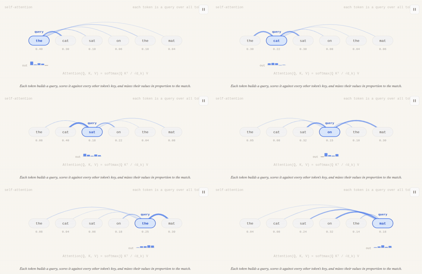
The step-by-step mathematical and logical pipeline of self-attention relies on three distinct vectors calculated for each token:
- Queries (Q): what a token is currently looking for in other tokens, the questions it asks of them.
- Keys (K): what kind of information a token holds, what it imparts to others.
- Values (V): how much weight should be given, how much information should be carried forward.
In simpler words: when a new token comes in, it "queries" against the existing tokens' "keys" in the context; the resulting dot-product, a similarity or attention score, is then weighted by each token's "value" vector to decide what's more important. The softmax function turns these raw scores into a row-wise probability distribution. Put simply, each token's output is just a weighted blend of every value vector in the sequence.
Formula 3.
Here $d_k$ represents number of embedding dimensions for each token.
Need for $\sqrt{d_k}$? Dot products are sums: $q \cdot k = \sum_{i=1}^{d_k} q_i k_i$ , one term per dimension. So a dot product is a sum over $d_k$ terms, and the more terms you add up, the larger that sum tends to get in magnitude (assuming each component is on a similar scale).
Left unchecked, this pushes the raw scores to grow with $d_k$ , and softmax reacts badly to that: it exponentiates each score before normalizing, so even a modest gap between the top score and the rest gets stretched into a much larger gap after exponentiating, and the top token's share balloons toward 1 while everyone else's shrinks toward 0. Dividing by $\sqrt{d_k}$ normalizes the variance back to approx. 1, which keeps the scores in a range where softmax can actually spread attention across multiple tokens instead of collapsing to one.
This is how few lines are required to code a Self-Attention block:
single_head_attention.py
class SingleHeadAttention(nn.Module):
      def __init__(self, d_model: int, d_k: int):
            super().__init__()
            self.d_k = d_k
            # PARAMETERS (learned); each weight: (d_k, d_model)
            self.W_Q = nn.Linear(d_model, d_k, bias=False)
            self.W_K = nn.Linear(d_model, d_k, bias=False)
            self.W_V = nn.Linear(d_model, d_k, bias=False)

      def forward(self, x: torch.Tensor) -> torch.Tensor:
            # x: (B, n, d_model)

            # ACTIVATIONS -- different for every input
            Q = self.W_Q(x)  # (B, n, d_k)
            K = self.W_K(x)  # (B, n, d_k)
            V = self.W_V(x)  # (B, n, d_k)

            scores = Q @ K.transpose(-2, -1)      # (B, n, n)
            scores = scores / self.d_k ** 0.5
            weights = scores.softmax(dim=-1)      # (B, n, n), rows sum to 1
            output = weights @ V                  # (B, n, d_k)
            return output

# B sequences, n = 3 tokens, d_model = 512, single head so d_k = d_model
attn = SingleHeadAttention(d_model=512, d_k=512)
x = torch.randn(B, 3, 512)                         # (B, 3, 512)
output = attn(x)                                   # (B, 3, 512)
Attention scores are often used as a window for explainability, since they show exactly which tokens a model leaned on to produce each output.
Take the sentence "My name is pranav": row-wise softmax turns each row of raw scores into a probability distribution over the keys, so every row below sums to 1, and each cell's shade encodes how much attention that query paid to that key:
pranav puts 55% of its attention back on name, more than double what it gives itself, while name and is each send 40% of their attention forward onto pranav. Expanding with Multi-Head Attention (MHA)
The intuition behind multi-head attention is that by applying the attention mechanism multiple times in parallel within its embedding space, the model can capture different types of relationships in the data.
MHA splits the embedding dimension into n_heads, each with d_model//n_heads dimension. Each of these heads has its own Q,K,V linear layers and perform their scaled dot-product attention independently. Each head attends to the sequence differently, letting the model capture several types of relationships at once instead of just one. A final projection linear layer W_O is required to project back the concatenated output of the heads to same shape as input.
multi_head_attention.py
class MultiHeadAttention(nn.Module):
      def __init__(self, d_model: int, num_heads: int):
            super().__init__()
            assert d_model % num_heads == 0
            self.d_model = d_model
            self.h = num_heads
            self.d_k = d_model // self.h

            # one projection for all heads; each weight: (512, 512)
            self.W_Q = nn.Linear(d_model, d_model, bias=False)
            self.W_K = nn.Linear(d_model, d_model, bias=False)
            self.W_V = nn.Linear(d_model, d_model, bias=False)
            self.W_O = nn.Linear(d_model, d_model, bias=False)

      def forward(self, x: torch.Tensor) -> torch.Tensor:
            B, n, _ = x.shape   # (B, 3, 512)

            Q = self.W_Q(x)     # (B, n, d_model) -> (B, n, d_model)
            K = self.W_K(x)
            V = self.W_V(x)

            # split into heads: (B, n, d_model) -> (B, h, n, d_k)
            Q = Q.view(B, n, self.h, self.d_k).transpose(1, 2)
            K = K.view(B, n, self.h, self.d_k).transpose(1, 2)
            V = V.view(B, n, self.h, self.d_k).transpose(1, 2)

            # scaled dot-product attention, all heads at once
            # (B, h, n, d_k) @ (B, h, d_k, n) -> (B, h, n, n)
            scores = (Q @ K.transpose(-2, -1)) / self.d_k ** 0.5
            weights = scores.softmax(dim=-1)

            # (B, h, n, n) @ (B, h, n, d_k) -> (B, h, n, d_k)
            out = weights @ V

            # concat heads: (B, h, n, d_k) -> (B, n, d_model)
            out = out.transpose(1, 2).contiguous().view(B, n, self.d_model)

            return self.W_O(out)   # (B, n, d_model)

# B sequences, n = 3 tokens, d_model = 512, h = 4 heads
mha = MultiHeadAttention(d_model=512, num_heads=4)
x = torch.randn(B, 3, 512)   # (B, 3, 512)
output = mha(x)              # (B, 3, 512)
Emergence of Multi-Query Attention (MQA)
MQA was brought into existence by Noam shazeer with "Fast Transformer Decoding: One Write-Head is All You Need" paper in 2019, which keeps multiple query heads but collapses K and V down to a single, shared key and value head, significantly reducing the memory load and speeding up inference.
Surprisingly the paper demonstrated that accuracy drop was minimal while the efficiency gains were huge. While naive pytorch implementation of MQA repeats the K and V heads to attend with multiple heads of Q but in reality all LLM engines efficiently handle this in cuda kernels thus saving memory bandwidth. MQA came as a saviour for the AI world which heavily relied on KV cache.
But What Is a KV Cache?
If you've come across prompt caching or context caching in Claude's or OpenAI's pricing pages, this is the principle underneath it: reusing cached K/V vectors instead of recomputing them is what lets long, back-and-forth conversations get up to 90% cheaper on repeat calls.
Autoregressive decoding, another name for next-token prediction in LLMs, generates one token at a time. At every step, the token currently being processed is turned into Q, K, and V vectors through the W_Q, W_K, and W_V weight matrices, then Q is multiplied by KT and the result is multiplied by V.
in Q · KT, each row of Q gets dotted against every column of KT. A row of Q corresponds to one token, so that row is the token currently being predicted for, scored against its own key and every past token's key. Once a token has been processed, its key and value vectors are fixed; nothing about generating the next token alters an earlier token's K or V.
A naive decoder that reprocesses the whole sequence from scratch at every step ends up computing each earlier token's K/V again and again, once per later step, for O(N²) K/V computations across a full decode. With caching, each token's K/V is computed exactly once, the moment it's first seen, and just looked up afterward in O(1), for O(N) total. Only the newest token's Q, K, and V get computed fresh at each step; everything already in the cache is reused as-is.What we are gaining in efficiency by doing less computations we are losing in memory by saving these KV caches.

Memory and Compute Footprint: Self-Attention vs. MHA vs. MQA
Attention blocks contribute majority of the LLM architectures, so optimizing the attention op greatly reaps benefits in inference efficiency.
Compute footprint
Self attention and MHA use the same amount of FLOPS for Q, K, V vector computation since we are just splitting the embedding dim into h heads. The final output vector in the attention block computed by the projection matrix W_o is where MHA adds the extra embedding_dim × embedding_dim MACs (MACs = multiply-accumulates, 1 FLOP = 2 × MACs).
For MQA, it's the same as MHA for the Q vector, but since we only use 1 head for K and V, each takes embedding_dim × (embedding_dim / n_heads) MACs. The projection matrix W_o computation remains identical for MQA and MHA.
Some napkin math:
d = embedding dim, h = heads
| Variant | W_Q | W_K | W_V | W_O | Total MACs |
|---|---|---|---|---|---|
| Self-Attention | d² | d² | d² | none | 3d² |
| Multi-Head Attention (MHA) | d² | d² | d² | d² | 4d² |
| Multi-Query Attention (MQA) | d² | d²/h | d²/h | d² | 2d² + 2d²/h |
Table 1. Compute cost (MACs) by attention variant.
Note: for multiple heads, h × (d × d/h) = d².
Other than this, the remaining FLOPs come from attention score computation, which is dot-products + weighted-sum MACs (for a full sequence of length n tokens, one layer): 2n² · d.
How 2n² · d: QKT computes the raw score between every query and every key: there are n queries and n keys, so n × n = n² dot products, and each dot product is between two d-dimensional vectors, d multiply-accumulates (MACs) each, for a total of n² · d MACs. softmax(QKT) · V is the weighted sum over values: for each of the n output positions, you're computing a weighted sum of n value vectors, each d-dimensional, the same shape as above, n positions × n values × d dims = n² · d MACs.
So it's identical across all three, regardless of how many heads or whether K/V are shared. Even true for MQA, since all h query heads still run their own separate score computation against the shared K/V.
With KV cache, we don't need to recompute every past token's K/V again at every step, we also pass only the new token through W_Q, W_K, W_V, not the entire token length N, so the cost comes down from O(N²) to O(N).
For the attention-score computation, instead of one 2n² · d pass over the whole sequence, decoding does one new query row scored against the t cached keys at each step: O(t · d) MACs, linear in however long the cache has grown, not quadratic.
Memory footprint
The real difference between the three isn't compute, it's the KV cache: how much has to be kept around and re-read at every decoding step.
| Variant | Query heads | KV heads | KV cache per token per layer |
|---|---|---|---|
| Self-Attention (single head) | 1 | 1 | 2d |
| Multi-Head Attention (MHA) | h | h | 2 × h × d_k = 2d |
| Multi-Query Attention (MQA) | h | 1 | 2 × d_k = 2d / h |
Table 2. KV cache memory footprint by attention variant.
KV cache size of MHA and self-attention is the same, since separate per-head K/V projections still add up to d embedding dimensions. The total cache size is 2 × b × n × d_h × n_h × L, where n = sequence length, L = layers, 2 is K and V together, d_h is head dim, n_h is the number of KV heads, and b is bytes per element (2 for fp16, 1 for int8).
Let's put in actual numbers: assume a 32k sequence/context length request sent to an LLM with 8 MHA blocks, d_h = 256, n_h = 8 KV heads, running in fp16 precision:
2 × 2 × 32,768 × 256 × 8 × 8 = 2,147,483,648 bytes ≈ 2 GiB of KV cache, for a single request (batch = 1).
This amount of GB space will be used by the KV cache along with the model parameters sitting in HBM of your GPU. You can see this going out of hand very quickly, and that's before multiplying by concurrent requests. The same setup with MQA (n_h = 1) needs 1/8 of that: 256 MiB instead of 2 GiB.
KV cache turned the token decoding step from compute bound to memory bound. MQA turned the problem from memory bound to bandwidth bound, the time required to move the KV cache in and out of HBM.
Tokenizer vs. Embedding Table
The tokenizer and embedding table sit at the very top of the architecture.
Tokenizer: Text → Token IDs
The tokenizer's job is to convert text into a numerical representation the model can work with, a simple lookup. A fixed vocabulary (257,152 entries) splits text into subword pieces and maps each one to an integer:
"a cat" → [235, 8055]
Embedding Table: Token IDs → Vectors
The embedding table (or embedding layer) converts each token ID from the tokenizer into vector form for the model to work on. embed_tokens is nn.Embedding(257152, 2048), a lookup table where the token ID is simply the row index:
[235, 8055] → [[0.12, -0.34, ...],   # 2048-dim vector for token 235
               [0.87,  0.21, ...]]   # 2048-dim vector for token 8055
paligemma_processor.py
class PaliGemmaProcessor:
      '''Responsible for text to tokens and processing images into pxs,
      and also return attn mask
      '''
      IMAGE_TOKEN = "<image>"

      def __init__(self, tokenizer, num_image_tokens, image_size):
            super().__init__()
            self.image_seq_length = num_image_tokens
            self.image_size = image_size
            tokens_to_add = {"additional_special_tokens": [self.IMAGE_TOKEN]}
            tokenizer.add_special_token(tokens_to_add)
            EXTRA_TOKENS = [
                  f"<loc{i:04d}>" for i in range(1024)
            ]  # These tokens are used for object detection (bounding boxes)
            EXTRA_TOKENS += [
                  f"<seg{i:03d}>" for i in range(128)
            ]  # These tokens are used for object segmentation
            tokenizer.add_tokens(EXTRA_TOKENS)
            self.image_token_id = tokenizer.convert_tokens_to_ids(
                  self.IMAGE_TOKEN
            )
            tokenizer.add_bos_token = False
            tokenizer.add_eos_token = False

            self.tokenizer = tokenizer

      def __call__(self, text, images, padding='longest', truncation=True):
            pixel_values = process_images(
                  images, size=(self.image_size, self.image_size),
                  resample=Image.Resampling.BICUBIC,
                  rescale_factor=1 / 255.0,
                  image_mean=IMAGENET_STANDARD_MEAN,
                  image_std=IMAGENET_STANDARD_STD,
            )
            pixel_values = np.stack(pixel_values, axis=0)
            pixel_values = torch.tensor(pixel_values)
            input_strings = [
                  add_image_tokens_to_prompt(
                        prefix_prompt=prompt,
                        bos_token=self.tokenizer.bos_token,
                        image_seq_len=self.image_seq_length,
                        image_token=self.IMAGE_TOKEN,
                  )
                  for prompt in text
            ]
            inputs = self.tokenizer(
                  input_strings,
                  return_tensors='pt',
                  padding=padding,
                  truncation=truncation,
            )
            return {'pixel_values': pixel_values, **inputs}
The PaliGemmaProcessor class converts input image and input text into pixel values and text tokens respectively. Since it wraps a Gemma 2 tokenizer, it also adds <image>, <seg>, and <loc> tokens, for handling image, segmentation, and detection/location tokens in input or output text. The add_image_tokens_to_prompt helper is where the actual prompt string gets built: 256 <image> placeholders first, then BOS, then the raw prompt, then a newline: [image tokens..., BOS, prefix tokens..., SEP, ...]
Weight Tying
This concept was new to me, and it stuck. Right after the tokenizer, an embedding table converts token IDs into vectors: (batch, seq_len) → (batch, seq_len, embed_dim). At the very end of the network sits a mirror-image layer that does the opposite: it takes those processed vectors and converts them back into token IDs. Both are doing a similar operation, on similar-shaped weight matrices: embed_tokens.weight, shape (257152, 2048), for the lookup, and its transpose, embed_tokens.weight.T, shape (2048, 257152), for the reverse. It turns out they use the same weight matrix.
If you go back to the Gemma-2B architecture, you'll notice an additional step right after the embedding layer: embedding scaling. nn.Embedding initializes from N(0, 1), small values, roughly −3 to 3. Logits computed directly at that scale would sit near zero and be hard to distinguish, so embeddings are multiplied by √hidden_size ≈ 45.3 right after lookup, bringing the shared matrix up to the scale the rest of the network (and the output logits) actually need.
Positional Embeddings
Both SigLip Vision encoder and Gemma 2B has a component called Position embedding which is added to token embedding. Self-attention on its own has no notion of order. It's just a weighted sum over the sequence based on content similarity. Shuffle the input tokens and the attention scores shuffle right along with them. It would treat "the dog bit the man" and "the man bit the dog" as the same bag of tokens. So positional information needs to be injected into tokens before the attention op.
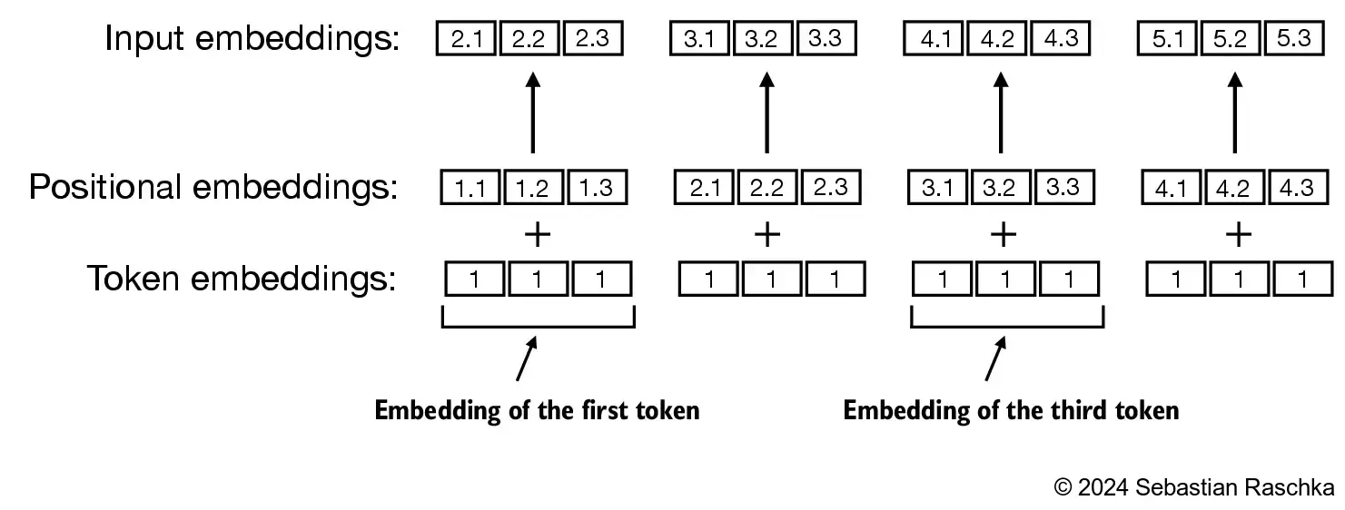
Absolute Positional Embeddings
Absolute positional embedding can further be classified into 2 categories:
- Learned: embedding vectors are initialized randomly and trained during training, one per position index. SigLIP's vision embeddings work exactly this way: a learned
position_embeddingtable with one entry per patch index, added to the patch embedding at the very start.self.position_embedding = nn.Embedding(num_positions, embed_dim) # one row per patch index, added to the patch embedding embeddings = patch_embeds + self.position_embedding(position_ids) - Fixed (sinusoidal): introduced in the original Attention Is All You Need paper: sine and cosine functions of different frequencies create a unique pattern per position, with no parameters to learn at all:
Formula 4.
$$PE(pos, 2i) = \sin\left(\frac{pos}{10000^{2i/d}}\right) \quad \text{for even indices}$$ $$PE(pos, 2i+1) = \cos\left(\frac{pos}{10000^{2i/d}}\right) \quad \text{for odd indices}$$
I found this great explanation on this by Nick Gustafson:
Each dimension gets a sine or cosine wave, and the frequency decreases as you move to higher dimensions. The low-order dimensions oscillate fast, changing rapidly from position to position. The high-order dimensions oscillate slowly, barely changing across dozens of positions.
The intuition I find most helpful is the clock analogy. A clock has a second hand (high frequency, fine resolution), a minute hand (medium frequency), and an hour hand (low frequency). Together the three hands uniquely identify any time within a 12-hour cycle. Sinusoidal encodings work the same way: the combination of different-frequency waves produces a unique fingerprint for each position.
Both encodings share the same limitation that a fixed-size table (or a formula tied to an absolute index) only ever encodes that a given token is at a position but says nothing how its position is relative to other tokens, this forces the model to work this relationship indirectly using two absolute numbers and neither generalizes past whatever length it was built for.
Since we are adding position information into actual token's content, the model has to learn to disentangle "what token is this" from "where does it sit" out of a single combined vector.
Relative Positional Embeddings
Positional embeddings are required by only 1 op in the transformer i.e attention block and within the attention block -- the attention score computation, specifically for the purpose to guide which token to attend based on their position and content.
So Relative position representation introduced by Shaw et al.'s Self-Attention with Relative Position Representations, later popularized by Press, Smith, and Lewis, "Train Short, Test Long: Attention with Linear Biases Enables Input Length Extrapolation", short for ALiBi. It directly injects the relative bias to the dot-product operation.
Formula 5.
Where i = query position and j = key position, m = the slope for each head. Since m changes per head, for some head larger values of m accentuate the i−j difference, forcing that head to attend in a more local window, while smaller m values are less punishing and allow for longer ranges.
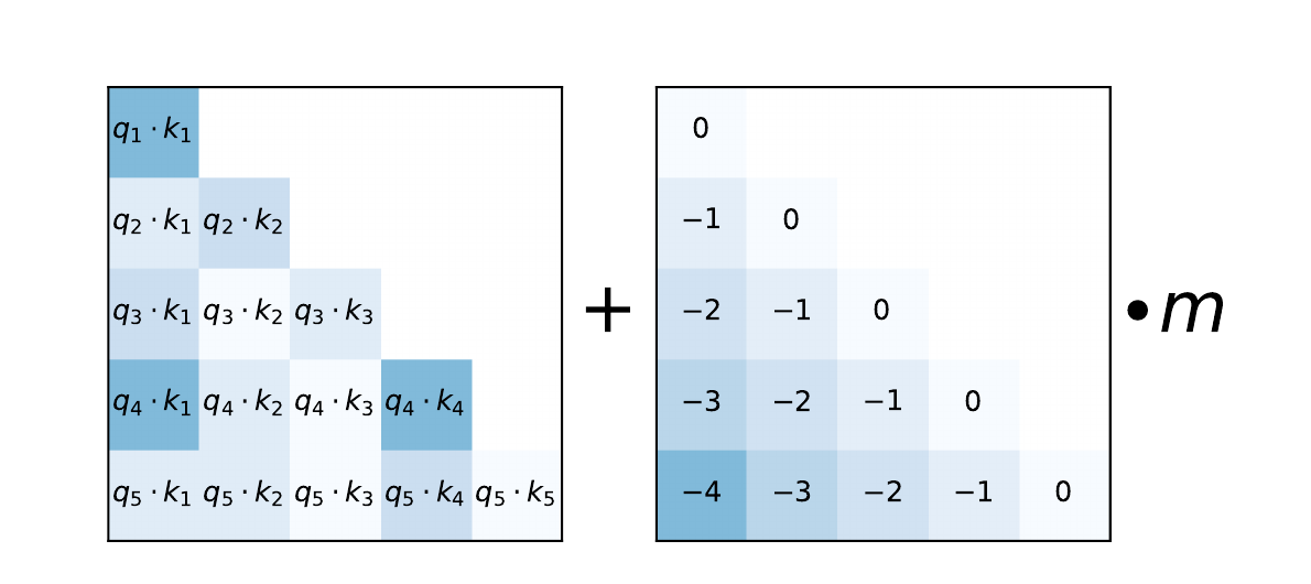
m, before the softmax. Figure 3 from Train Short, Test Long (Press, Smith & Lewis, 2022).Fig. 24 shows how this plays out during multi-step decoding: at timestep i=2, query q2 can only look at the current key k2 and the earlier key k1, and the positional bias tells it that k1 sits one token position behind.
Relative positional embeddings are applied at each attention block, so they stay fresh at every layer and don't get disentangled from content the way fixed (absolute) positional embeddings can in later layers of the network. ALiBi is simple to implement and extrapolates well to longer contexts, but far-off tokens always receive a penalty. The model can still attend to them if the raw attention score is high enough, it just has to overcome the bias to do so.
Rotary Positional Embedding (RoPE)
RoPE (Su et al., 2021) combines benefits of both absolute and relative embeddings by rotating Q and K vectors in a high-dimensional space; the amount of rotation depends on the token's position in the sequence. The embedding itself is left alone, no addition.
Given a token, RoPE rotates its key and query vectors by multiplying them with a rotation matrix based on the token's position. The rotated vectors then feed into attention exactly as usual (dot product, then softmax); nothing else in the transformer changes.
The mechanism is straightforward: pair up the dimensions of the query vector, (q0, q1), (q2, q3), (q4, q5), and so on. Each pair lives in its own 2D plane, and each one gets rotated independently:
Formula 6.
Mathematical Proof of Relativity
Now let's prove that RoPE is relative: that the attention score between two tokens depends only on their relative positions, not their absolute positions.
Define the RoPE operation as rotating a projected vector by an angle proportional to its position, where x is the projected query or key vector, θ is that dimension pair's fixed rotation frequency, and m is the token's position in the sequence:
Consider two tokens at positions m and n:
We calculate the attention score as their dot product, and expand it:
Rotation matrices have the nice property that:
Therefore the attention score becomes:
As you can see, the score is a function of the relative position only, the difference between m and n, and never depends on their absolute values.
The magic is in the dot product. When you compute q(posm) · k(posn), the two rotation matrices partially cancel. What survives depends only on the difference m−n. So RoPE naturally encodes relative position, which is exactly what attention cares about.
Rotation Matrix for Higher Dimensions
More often than not, the embedding dimension of the model is not 2; it's often much larger. So how does the rotation matrix change? The RoFormer paper's authors proposed the following composition: for position m and embedding dimension d, the rotation matrix is composed of d/2 independent 2×2 rotation blocks, each rotating a different pair of dimensions at its own frequency θi. Since this construction is sparse (block-diagonal, mostly zeros), the authors recommend a computationally efficient way to compute its product with a token embedding vector x, without ever building the dense matrix:
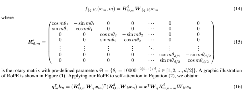
RΘ,m, and the proof that qmTkn collapses to a function of n−m alone. From RoFormer: Enhanced Transformer with Rotary Position Embedding (Su et al., 2021).Each block's frequency θi is fixed (not learned), and decreases geometrically with the dimension-pair index, the same base-10000 scheme sinusoidal encoding uses:
Formula 7.
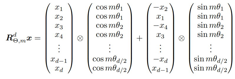
x with the cosines, plus one element-wise product of a "rotate-half" reordering of x with the sines, exactly the form used by Gemma's GemmaRotaryEmbedding in this codebase.The above rotation matrix can be simplified into this form, and just with this simple formula you embed m's position into an x vector of d dimensions. Both K and Q vectors are rotated using RoPE at every attention op.
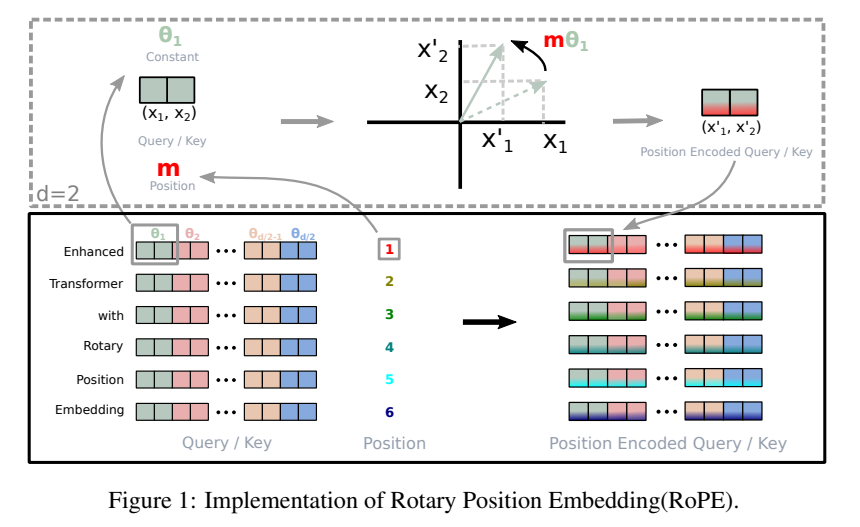
mθi, and every token in the sequence ends up with its own distinct, position-encoded Q/K vector.Advantages of RoPE
- Combines absolute and relative. Each token is still rotated by an angle tied to its own absolute position
m, but the resulting attention score collapses to a function ofn−malone, getting us the desired relative properties. - Extrapolates to longer sequences. RoPE along with techniques like NTK-aware scaling and YaRN scales well for longer contexts during inference. They work how to modulate the frequency of different dimensions of distant positions to positions known to model.
- Just like ALiBi, RoPE plays naturally with the KV cache. RoPE rotates
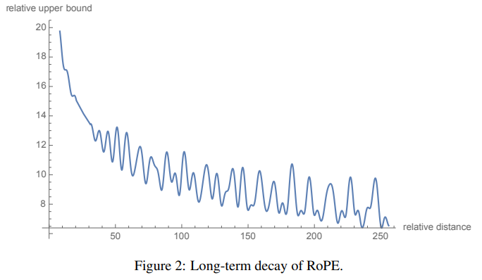
QandKusing each token's own absolute position index, computed once when that token is first processed. We can store this rotatedKin cache and keep on using it. - Long-term decay. Because RoPE rotates each dimension pair at a different frequency and then sums their contributions, the terms for distant token pairs increasingly land out of phase with each other and partially cancel, so the upper bound on the inner product between two RoPE-rotated vectors shrinks as their relative distance grows. Meaning distant tokens received less weightage during attention. This was a nice property that authors discovered.
Attention Mask
Before transformers and LLMs, there were RNNs and LSTMs, which relied on hidden states leading up to the final predicted token. Training an RNN looked like: process token 0, produce a hidden state; process token 1, produce a new hidden state; and so on. Each step depends on the previous step's output. RNNs' biggest drawback was their inability to parallelize, leaving the GPU underutilized. Even though loss was computed for each step, the training process was inefficient: it can't compute all these hidden states simultaneously, because the inputs to later steps aren't ready yet.
The above interaction shows the training of a 1-layer RNN. At each timestep, the RNN requires the old hidden state and the token at time t to predict the next token, updating the hidden state. So even though we've parallelized the tokens in a batch to go through the RNN cell and update hidden states for the entire batch [ht,0, ht,1, ... ht,n] (where t is the timestep and n is the batch element index), the next column, the next timestep, can't begin processing until the computations for its last timestep are done. This dependency is what makes it slower to train.
Transformers and their self-attention mechanism allow a token to look at other tokens in the context. The current token being predicted can attend and look at all past tokens via its attention op, no hidden states, no waiting on the last token to be generated.
Transformers train for autoregressive decoding by feeding it a sentence and asking it to predict the next token at each token step.
Transformers allow parallelism at each token step, so all tokens can produce the next token efficiently in one forward pass rather than sequentially like in RNNs. All token steps produce a loss after one forward pass.
Hover a predicted token to see which input row produced it.
| inputs: | The | cat | sat | on | it |
| targets: | cat | sat | on | it | . |
| predictions: | cat | sat | on | it | . |
Since we're training for next-token prediction, targets are inputs shifted by one token, shown above. With 5 input tokens, we predict at all 5 positions at once. With the mask off, cat's query attends over the whole sentence, including “sat”, “on”, and “it”, the tokens it's supposed to predict. That's not prediction, it's reading the answer during the attention op.
The causal mask stops this. Position i can only attend to itself and earlier positions, never i+1 or beyond. With the mask on, “cat” sees only “The” and itself, so it has to make educated guesses rather than peek ahead, which is what forces the model to actually learn.
The mask works directly on the raw dot products: it sets every future-token score to -∞, so once softmax runs, those positions get exactly zero weight.
Training an LLM on next-token prediction doesn't require explicit labelled data. It's self-supervised: the target is that same input sequence shifted right by one.
input:  [BOS, "The", "cat", "sat", "on", EOS]
target: ["The", "cat", "sat", "on", EOS]   ← input shifted right by one
Because the causal mask guarantees position i's logits depend only on tokens ≤ i, a single forward pass produces a usable prediction at every position, not just the last one. So every token in the sequence contributes a training signal except the very last one, whose logits would be predicting whatever comes after EOS, a token this example simply doesn't have. Cross-entropy loss is averaged over all the positions that do have a target:
Formula 8.
next_token_loss.py
logits = model(input_ids)                        # [B, seq_len, vocab]
loss = cross_entropy(
    logits[:, :-1, :],   # every position except the last (EOS has no target)
    input_ids[:, 1:],    # the actual next token at each of those positions
)
What about during inference? During inference, we anyways don't have future tokens, we're predicting it token by token. So inference doesn't require causal masking.
(Note : only if the LLM were to predict from very first token.)
Prefill vs. Decode
Generation is never a blank slate: it's built on top of the prompt the user gives, a question, an instruction, anything. Prefill is one parallel forward pass over that whole prompt: it builds the KV cache and produces the first token's logits, exactly like training. Decode then generates one token at a time with n forward passes, reusing that cache.
Prefill needs a causal mask: it computes every prompt position in one pass, so without the mask, position i's cached key/value would encode information from positions after it, corrupting every later decode step that attends back to it. Decode needs no mask: each step has only one query token, and no future tokens exist yet to leak from.
How PaliGemma Does Masking
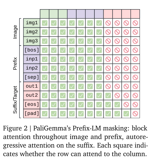
PaliGemma's prompt looks different from a normal decoder-only LLM's: [image tokens, BOS, text tokens, SEP]. It uses Prefix-LM masking: no causal mask during prefill, so image tokens are allowed to attend to the text tokens that come after them in the prompt. This lets the image tokens' attention be shaped by the task at hand, detection, OCR, whatever the prompt asks for, so vision features are conditioned on the task before generation ever begins.
Special Tokens
Object Detection: Location Tokens
PaliGemma has no bounding-box regression head, no anchor boxes, no NMS, no Hungarian matching, none of the machinery in Faster R-CNN/YOLO/DETR.
Section 3.1 of the paper: "During PaliGemma's pretraining, we limit ourselves to 'text' covering natural language, object detection, and instance segmentation, but this API remains versatile."
A bounding box is just another string the decoder autoregressively generates: 1024 vocabulary tokens, each one bin of a 1024-way discretization of a normalized image coordinate ([0,1] split into 1024 bins).
A box is 4 tokens, y_min, x_min, y_max, x_max:
"detect cat" → <loc0120> <loc0200> <loc0450> <loc0600> cat
                 y_min     x_min     y_max     x_max   entity
At inference:
decode a <locXXXX> token
→ bin index 0–1023
→ divide by 1024
→ normalized coordinate in [0,1]
→ multiply by the checkpoint's actual pixel resolution (224/448/896)
→ pixel coordinate
Segmentation: Segment Tokens
As paper mentions: "We also add 128 VQVAE tokenized single-object mask tokens (<seg000> to <seg127>) to support referring expression segmentation."
A paligemma segmentation example output format:
"<loc0347><loc0553><loc0788><loc0749><seg093><seg106>...<seg127><seg121>;cat"
 └────────location tokens─────────┘└───────segmentation tokens───────┘└entity┘
4 <loc> tokens (bounding box) plus 16 <seg> tokens (mask) per object.
PaliGemma uses a VQ-VAE trained to compress segmentation masks: an encoder maps the mask to continuous latent vectors, each is quantized to its nearest codebook entry, and a decoder reconstructs the mask from those quantized vectors. The 128 codebook entries are exactly PaliGemma's <seg000>–<seg127> tokens.
At inference, PaliGemma generates left to right: first the bounding box (<loc0347><loc0553><loc0788><loc0749>), then 16 <seg> tokens (<seg093><seg106>...<seg121>), one per codebook index. The VQ-VAE then looks up each index's codebook vector, arranges the 16 vectors into the 4×4 latent grid, and decodes them into a binary mask, which gets placed inside the predicted bounding box.
Training Stages / Phases
PaliGemma's training is split into 4 stages:
Stage 0
Unimodal Pretrain
Off-the-shelf checkpoints, nothing custom.
SigLIP-So400m + Gemma-2B, pretrained separately, reused as-is.
Stage 1
Multimodal Pretrain
Train everything, broad task mixture, 224px, 1B examples.
Model understands images + text broadly, but only at 224px resolution.
Stage 2
Resolution Increase
Continue pretraining at higher res: 448px +50M / 896px +10M examples.
Model handles small text/objects, fine detail at 448px/896px.
Stage 3
Transfer
Fine-tune per downstream task, all params tunable.
Task-specific specialist checkpoints (COCOcap, RefCOCO, NLVR2, ...).
Stage0: Unimodal Pretraining
No custom pretraining, just reuse two already-trained checkpoints:
- SigLIP-So400m ("shape optimized" ViT), contrastively pretrained via sigmoid loss.
- Gemma-2B v1.0, raw pretrained checkpoint.
Stage1: Multimodal Pretraining
Combines the two unimodal models and trains the whole model: nothing frozen, including the image encoder. As mentioned in the PaliGemma paper, contrary to common practice (e.g. LiT) of freezing the image encoder here, PaliGemma keeps it trainable, following CapPa/LocCa findings that captioning objectives teach the encoder spatial/relational skills that contrastive pretraining (CLIP/SigLIP-style) misses.
A slow linear warm-up on the image encoder's learning rate avoids destructive gradients from the initially-misaligned LLM.
Trained on a broad mixture of tasks, each prefixed by task type so skills don't conflict:
caption {lang}, ocr, answer en {question}, question {lang} {English answer}, detect {thing};{thing};..., segment {thing};{thing};..., caption <ymin><xmin><ymax><xmax> (grounded captioning).
Run at 224×224 resolution (256 image tokens), text sequence length 128, for 1 billion examples: the goal at this stage is breadth of cross-task visual knowledge (concepts/cultures/languages).
Stage2: Resolution Increase
Stage1's 224px model can't handle small-object detection/segmentation or reading small text (charts/infographics/documents), so two further checkpoints are trained at higher resolution: 448×448 (+50M examples) and 896×896 (+10M examples).
Same task mixture as Stage1, but upweights resolution-sensitive tasks and allows longer suffixes (up to N_txt = 512) so e.g. OCR can request all text, detection/segmentation can request all annotated objects.
Stage3: Transfer
Fine-tune the Stage1/2 base checkpoints per-task on 30+ downstream benchmarks (COCO Captions, Remote Sensing VQA, Video Captioning, InfographicQA, multi-image NLVR2, bounding-box WidgetCap, etc.). All parameters are tunable, with a per-task hyperparameter sweep over resolution/epochs/LR/label-smoothing/dropout/weight-decay/freeze-ViT/beam-search.
A single "mix" checkpoint is also released, jointly transferred on a subset of tasks plus detailed captioning/long QA, described as "a step in the direction of" instruction tuning, but not full instruction tuning.
Why PaliGemma Is Not an Instruction-Tuned Model
PaliGemma differs from models like LLaVA or GPT-4-based ones, which are trained on (image, instruction, response) triples covering many task types phrased as natural instructions or conversations, rather than one fixed template per task. That training lets those models hold follow-up conversations after the initial prompt and answer. PaliGemma is an open base VLM without instruction tuning, a deliberate scope decision.
Results
Section 4 of the paper transfers PaliGemma to 30+ downstream benchmarks by fine-tuning, none of which are part of the pretraining mixture, their images are explicitly removed from the pretraining data, so these are genuine held-out evaluations. Table 1 reports scores for all three resolution checkpoints (224px, 448px, 896px) where applicable.
| Task | 224px | 448px | 896px |
|---|---|---|---|
| COCOcap (captioning) | 141.9 | 144.6 | — |
| VQAv2 | 83.2 | 85.6 | — |
| GQA | 65.6 | 67.0 | — |
| TextVQA | 55.5 | 73.2 | 76.5 |
| ChartQA (human) | 40.0 | 54.2 | 74.9 |
| RefCOCO (testA, segmentation) | 75.7 | 77.9 | 78.7 |
| RefCOCOg (test, segmentation) | 68.2 | 71.0 | 72.7 |
Table 3. A representative slice of the paper's own Table 1. Resolution-sensitive tasks like TextVQA and ChartQA gain the most from higher-resolution checkpoints; captioning and general VQA barely move.
Video tasks are evaluated only at 224px (16 sampled frames, each encoded separately): ActivityNet-QA 50.8, ActivityNet-CAP 34.6, MSRVTT-QA 50.1, MSRVTT-CAP 70.5, MSVD-QA 60.2, VATEX 79.7.
The paper highlights one result (Section 7, Noteworthy tidbits): "Our MMVP result is SOTA by a large margin. PaliGemma at 224px achieves 47.3% paired accuracy, while GPT4-V and Gemini achieve 38.7% and 40.7%, respectively, and all other models including LLaVa perform below chance."
Lingering Thoughts
Working in the medical domain, mostly with images, videos, and text, I find VLMs like PaliGemma genuinely appealing. But the question I keep coming back to: are these decoder-only architectures, trained on a grab-bag of cross-task data, actually good enough to replace battle-tested, purpose-built segmentation, detection, and landmark models?
If we're fine-tuning VLMs per task anyway to hit benchmark numbers, why not just fine-tune a dedicated segmentation encoder or YOLO detector instead?
Is the industry actually moving toward unified architectures, where boxes, masks, and text are all just tokens an LLM spits out, or is that still more promise than proof?
The paper doesn't help me answer this. It never benchmarks PaliGemma against dedicated single-task detectors or segmentation encoders, only against other VLMs (PaLI-X, PaLM-E). Its "state of the art" claims are relative to other VLMs, not to the specialist models it would actually need to beat to replace them.
Still, the model punches above its weight at 3B parameters, and the paper's ablations, on the image encoder, the connector design, whether to freeze the vision tower, are genuinely thought-provoking. If you want to implement it yourself, Umar Jamil's 5-hour walkthrough is an excellent guide to the mechanics, though it isn't production-ready: MQA isn't handled efficiently, and the image encoder reruns needlessly at every decode step.
My honest read: for a fixed, well-scoped task, a specialist model is still probably the safer bet. What a VLM buys you is flexibility, one model, prompted differently, doing detection, segmentation, and captioning without three separate pipelines.
Sources
- Noam Shazeer: Fast Transformer Decoding: One Write-Head is All You Need, arXiv:1911.02150 (2019)
- Sebastian Raschka: Build a Large Language Model (From Scratch), positional embeddings diagram, image source
- Su et al.: RoFormer: Enhanced Transformer with Rotary Position Embedding
- Umar Jamil: Coding a Multimodal (Vision) Language Model from scratch in PyTorch with full explanation, YouTube video
- Umar Jamil: companion project repo, github.com/hkproj/pytorch-paligemma
- Beyer, Steiner, Susano Pinto, et al.: PaliGemma: A versatile 3B VLM for transfer, arXiv:2407.07726
- Liu, Li, Wu, Lee: Visual Instruction Tuning (LLaVA), arXiv:2304.08485
- The Gustafson: Causal Masking, how the mask is applied: additive, before softmax