Echo(JEPA) and Its Origins
How Yann LeCun's bet against pixel prediction became the largest latent-predictive foundation model built for the heart.
How and by who?

Yann LeCun, JEPA's originator
JEPA (the Joint-Embedding Predictive Architecture) is the brainchild of Yann LeCun, formerly Meta's Chief AI Scientist. His vision is to create machines that can learn internal models of how the world works.
He argues the current generative models and training them with tasks to try to reconstruct every detail of a signal is wasteful and impossible since the actual world is inherently unpredictable and noisy(like LLMs with their pretraining step with next predicition token task).
He draws inspiration of how humans understand the world around them and learn from the environment in terms of abstract and high level representations and ignoring low level details most of the time.
He encourages to build strong foundational models around this thesis and these foundational models will have abstract knowledge of the environment, physics and planning . Later more specialized models can be built on top of this like action model for robots or text generation models like current LLMs.
What JEPA actually predicts
In JEPA, a model ingests a pair of related inputs;e.g. consecutive video frames or adjacent image patches and encodes each into an abstract representation. A predictor module then tries to predict the representation of the "target" input from the representation of the "context" input, bringing them closer in embedding space.
Unlike generative models, JEPA does not attempt to reconstruct every detail of the input; it works in an abstract embedding space, which lets it focus on high-level, essential information and ignore irrelevant or unpredictable details. The model can be viewed as an Energy-Based Model (EBM) operating on representations: it assigns low energy when the predicted representation matches the actual target representation, and high energy when they mismatch. The "joint embedding" part means both inputs are mapped into a common representation space where the prediction is made, rather than directly predicting raw data.
From an information-theoretic perspective, the goal is to capture as much predictable information as possible in the representations while discarding unpredictable noise. This involves a delicate balance between information preservation and compression: if the representation preserves nearly all information from the input, it may include lots of irrelevant or random detail that makes prediction difficult; if it compresses too aggressively, it may lose the structure needed to predict the target. In other words, JEPA seeks an abstraction level where the representation has high mutual information with both the input and the target, but low entropy in terms of irrelevant bits. LeCun's own example is video prediction: trying to predict every pixel of future frames is nearly impossible due to chaotic details like flickering leaves or textured surfaces.
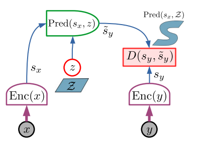
The main advantage of JEPA is that it performs predictions in representation space, so it doesn't need to predict every detail of y, and irrelevant details can be eliminated by the encoders. More precisely, the main advantage of this architecture for representing multi-modal dependencies is twofold: (1) the encoder function sy = Enc(y) may possess invariance properties that will make it produce the same sy for a set of different y, so the energy stays constant over that set and the model can capture complex multi-modal dependencies; (2) the latent variable z, when varied over a set 𝒵, can produce a set of plausible predictions Pred(sx, 𝒵) = {šy = Pred(sx, z) ∀ z ∈ 𝒵}.
If x is a video clip of a car approaching a fork in the road, sx and sy may represent the position, orientation, velocity and other characteristics of the car before and after the fork, respectively, ignoring irrelevant details such as the trees bordering the road or the texture of the sidewalk. z may represent whether the car takes the left branch or the right branch of the road.
Source: LeCun, A Path Towards Autonomous Machine Intelligence (2022), openreview.net/pdf?id=BZ5a1r-kVsf.
Self-supervised learning methods
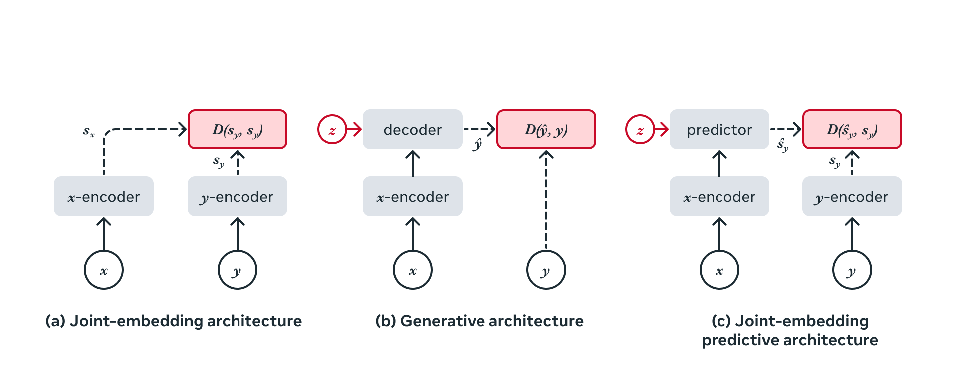
JEPA didn't invent self-supervised learning; it's a deliberate third option next to two established families, each having its drawback.
Source: LeCun, A Path Towards Autonomous Machine Intelligence (2022), openreview.net/pdf?id=BZ5a1r-kVsf.
Invariance-based (joint-embedding) methods
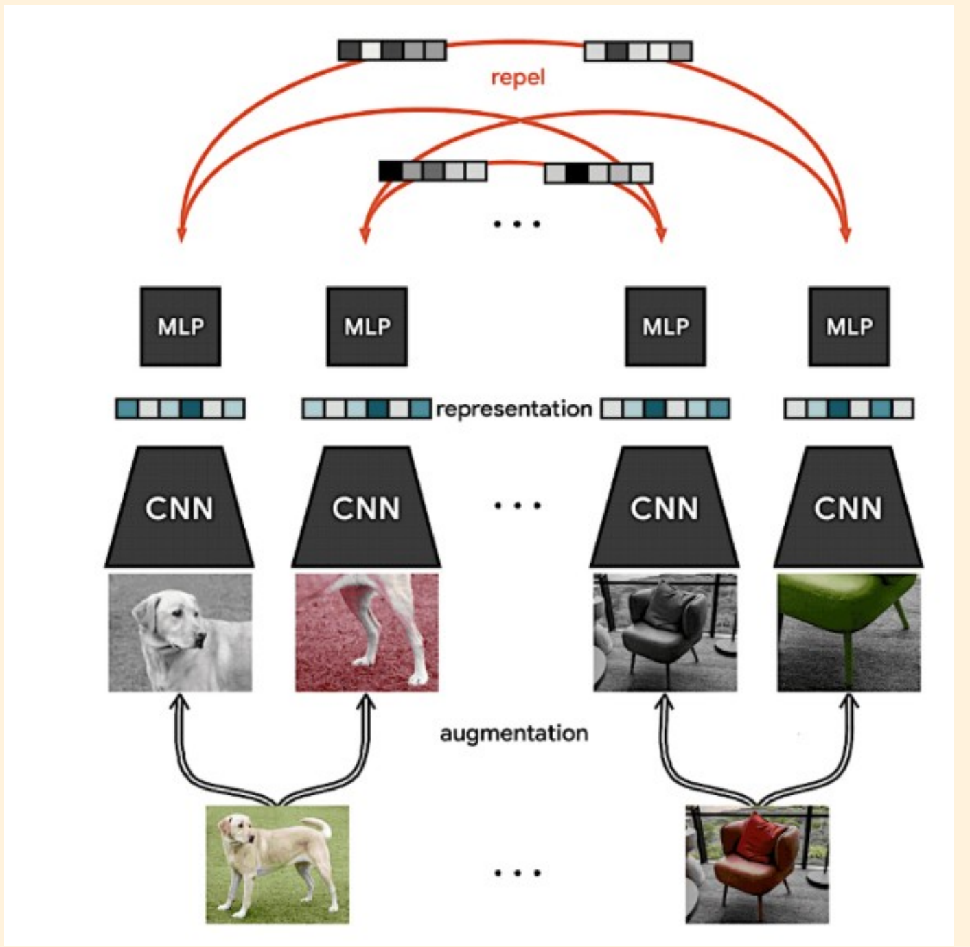
Train an encoder to output similar embeddings for different views of the same input, views constructed via hand-crafted data augmentations (random scaling, cropping, color jittering). The energy landscape is flat for compatible inputs (low energy regardless of what the encoder outputs), so these methods need tricks to prevent representation collapse, where the encoder ignores the input entirely.
Source: LeCun, A Path Towards Autonomous Machine Intelligence (2022), openreview.net/pdf?id=BZ5a1r-kVsf.
| Sub-type | Mechanism | Examples |
|---|---|---|
| Contrastive | Explicitly pushes apart embeddings of negative (incompatible) pairs | SimCLR, MoCo |
| Non-contrastive | Minimizes informational redundancy across embeddings | Barlow Twins, VICReg |
| Clustering-based | Maximizes entropy of the average embedding | SwAV |
| Asymmetric architecture | Asymmetric x-encoder / y-encoder design to avoid collapse | BYOL, SimSiam |
Table 1. Sub-types of invariance-based (joint-embedding) self-supervised methods.
Limitation: the hard-coded augmentation invariances may not transfer across tasks or modalities; image classification and segmentation don't need the same invariances.
Generative (reconstruction) methods
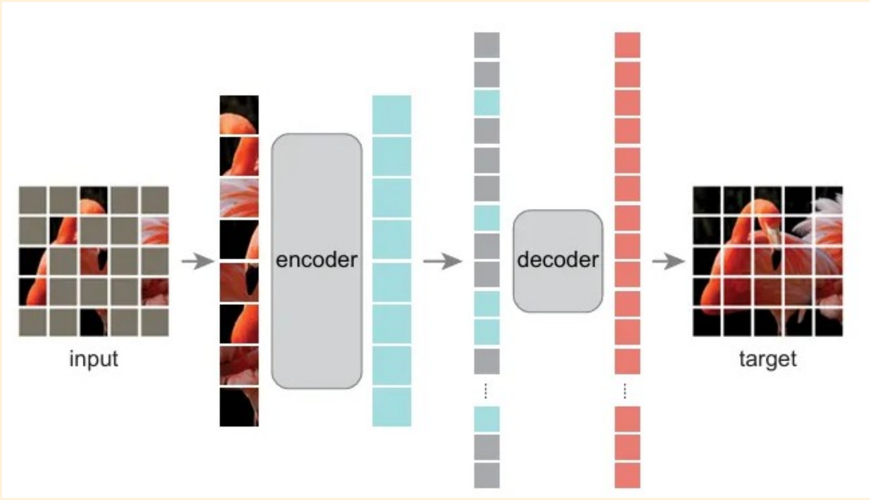
Learn to directly reconstruct signal y from a compatible signal x, using a decoder conditioned on a latent z. Reconstruction collapse isn't a concern here, since the informational capacity of z is kept low.
Source: LeCun, A Path Towards Autonomous Machine Intelligence (2022), openreview.net/pdf?id=BZ5a1r-kVsf.
| Method | What is z | Notes |
|---|---|---|
| MAE | Position tokens for masked patches | Encoder only sees visible patches |
| BEiT | Tokenized patch targets (dVAE) | Predicts discrete tokens, not pixels |
| SimMIM | Raw pixel values | Simple regression loss; no tokenizer or clustering needed |
| CAE | Encoder + decoder with alignment constraint | Enforces representation predictability |
| data2vec | Online target encoder representations | Predicts via masked encoder |
Table 2. Generative (reconstruction) methods, compared by what their latent z represents.
Limitation: because the loss is in pixel/token space, the model is penalized for every low-level mismatch, incentivizing it to model texture and noise rather than semantics.
I-JEPA: the first concrete implementation
I-JEPA (Image Joint Embedding Predictive Architecture) is the first concrete implementation of JEPA, for computer vision. The idea is to predict missing information in an abstract representation that's more akin to the general understanding people have, rather than in raw pixel space.
Compared to generative methods that predict in pixel/token space, I-JEPA uses abstract prediction targets, for which unnecessary pixel-level details are potentially eliminated, leading the model to learn more semantic features. A second core design choice guiding I-JEPA toward semantic representations is its multi-block masking strategy: predicting large blocks containing semantic information (at sufficiently large scale), using an informative, spatially distributed context.
Put simply: I-JEPA patchifies the input image, then masks out everything except one large, contiguous context block, and encodes that block with the context encoder. In parallel, the target encoder, an EMA copy of the context encoder that acts as its stable, slowly-updated twin, encodes the full image and produces representations for four independently sampled target blocks.
The predictor is then asked to predict each target block's representation using only the context encoder's representations, with the target encoder's actual representations serving as ground truth.
The way I read it: the two encoders' job is to compress the image down to high-level, semantically relevant representations, and asking the predictor to fill in information about most of the image from a limited context is what injects a generative, fill-in-the-blank pressure into the training objective.
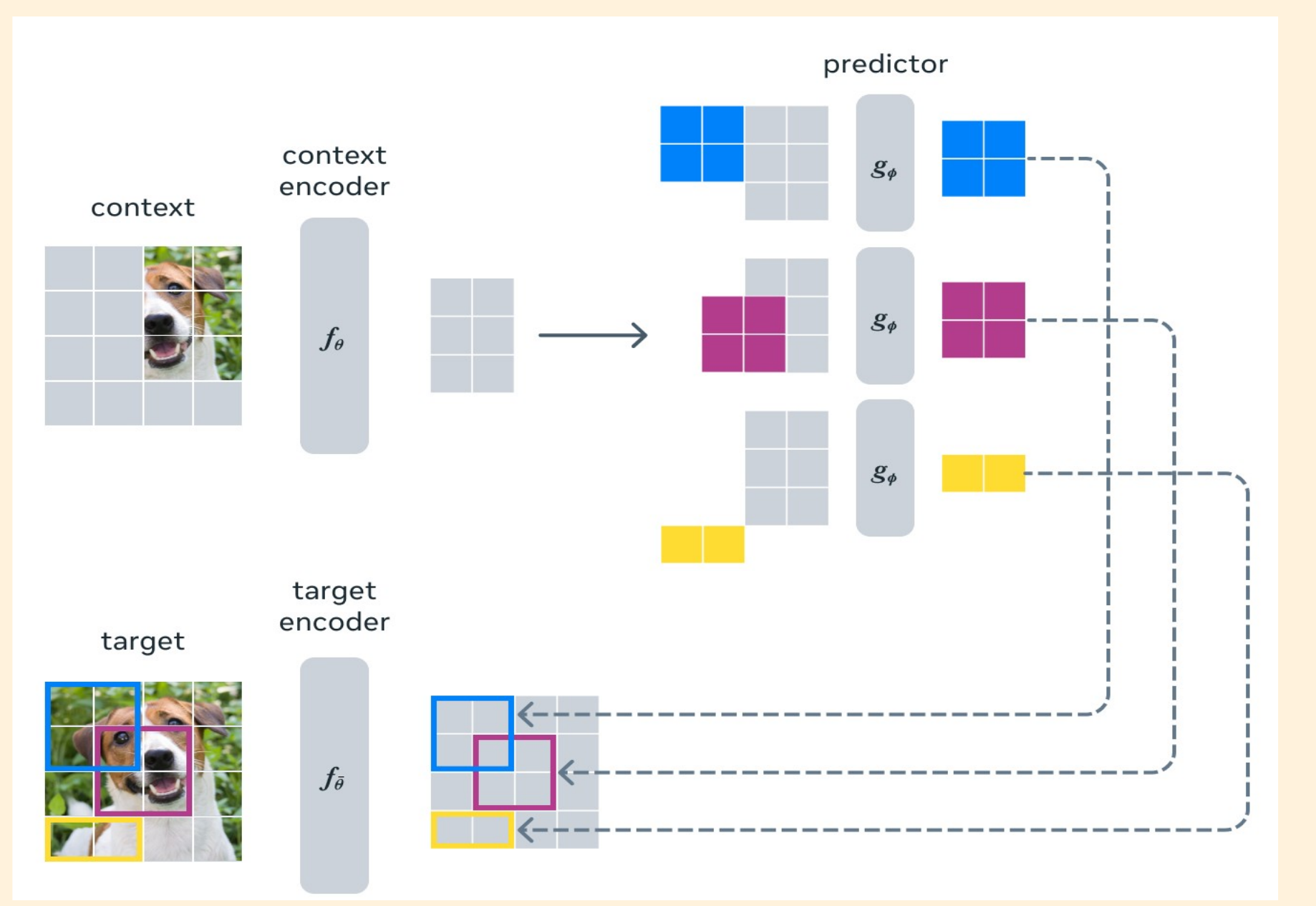
Source: Assran et al., I-JEPA: Self-Supervised Learning from Images with a Joint-Embedding Predictive Architecture (2023).
Architecture 1: I-JEPA Architecture
The figure above shows the concept; the actual forward pass moves through five components, each with its own tensor shapes. This is the original ViT-H configuration from the I-JEPA paper.
- Patchify
-
- 224×224×3 image → 16×16 grid of 14×14 patches (224 / 14 = 16 per side, 256 patches total)
- Each patch is flattened to 14×14×3 = 588 values
- Linearly projected to width 1280 via
Conv2d(3, 1280, kernel=14, stride=14), equivalent to oneLinear(588 → 1280)per patch - A sincos positional encoding is added elementwise (⊕) to all 256 tokens, before either branch splits off
- Context Block
-
- One region is sampled directly from the 16×16 patch grid: scale 0.85:1.0 of the image (almost the whole image), unit aspect ratio
- This crop happens before encoding: the context encoder only ever sees these patches, never the rest of the image
- Patches inside any of the four target blocks are removed, so the model can't trivially copy overlapping content; that leaves roughly N_ctx ≈ 220 of the original 256 patches
- The result is one large, spatially-distributed context region, not a scattering of isolated patches
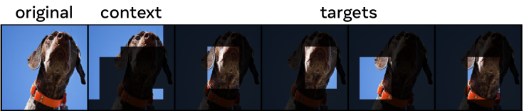
Figure 6. Sample of Context block and the 4 target blocks. - Context Encoder (f)
-
- Takes the sampled context block's patches, already carrying their positional encoding from the patchify step
- Passes through the full ViT-H: 32 layers, 16 attention heads of dimension 1280 / 16 = 80 each
- Output: context representations s_x ∈ ℝN_ctx × 1280
- Target Encoder (f_ema)
-
- Architecturally identical to the context encoder, and uses the same positionally-encoded tokens from the patchify step, so yes, it gets positional encoding too
- Weights are never touched by gradient descent, only by the exponential moving average shown below
- Encodes the full, unmasked 256-token image, unlike the context encoder, which only ever sees the sampled context block
- Output: full-image representations, 256 × 1280
- Target Blocks
-
- Four blocks are sampled independently: scale 0.15:0.20 of the image each, aspect ratio 0.75:1.5, roughly 38–51 patches per block
- Unlike the context block, target blocks are selected after the target encoder has already processed the full image, by reading the corresponding rows out of its full-image representation
- That ordering matters: the target encoder's representations are computed with full context, so they stay stable regardless of exactly where a target block lands
- Layer-normalized into target representations s_y ∈ ℝM × N_tgt × 1280, the actual prediction targets
- Predictor (g)
-
- Context representations are projected down:
Linear(1280 → 384). Yes, it gets positional encoding too, but a separate one from the encoders': the predictor works in a narrower 384-dim space, so it re-embeds positions at that width rather than reusing the 1280-dim encoding - One learned mask token per target patch is concatenated on, carrying only that same 384-dim positional embedding for where the patch sits: mask tokens carry no image content, only positional embeddings indicating which patches to predict
- Combined sequence runs through 12 layers of 16-head self-attention at width 384 (head dim 384 / 16 = 24), letting mask tokens attend to the visible context tokens
- Mask-token outputs are kept and projected back up:
Linear(384 → 1280), producing š_y - Bottleneck at 384-dim: the predictor is intentionally narrow (384 vs. 1280 in the encoder). It must be cheap since it runs M = 4 times per image, one per target block, and the bottleneck actually improves downstream performance
Architecture 2. Predictor in detail. - Context representations are projected down:
- Loss
-
$$D(\hat{s}_y, s_y) = \frac{1}{N_{\text{tgt}}}\sum \left\| \hat{s}_y - s_y \right\|_2^2$$
- Average squared L2 distance between predicted and target representations, computed only over the target patches
- Gradients update the context encoder and predictor only
- The target encoder is never backpropagated through: see the next section for exactly how it's updated instead
Target encoder EMA and the loss
- At the start of training, the target encoder is a direct weight copy of the context encoder: every parameter tensor duplicated (patch projection, positional embeddings, all 32 transformer layers).
- Each training step has two phases: the context encoder gets a gradient update, then the target encoder gets an EMA update:
$$\theta_{\text{ema}} \leftarrow m \cdot \theta_{\text{ema}} + (1 - m) \cdot \theta_{\text{context}}$$
- θema is the current theta value, m is the momentum, θcontext is the new context-encoder value. With m = 0.996, that's a weighted average of all past context-encoder states, with exponentially decaying weights for older states:
$$\theta_{\text{ema}} \leftarrow 0.996 \cdot \theta_{\text{ema}} + 0.004 \cdot \theta_{\text{context}}$$
- Momentum doesn't stay fixed: it ramps linearly from 0.996 to 1.0 over the full training run.
- Early in training (m = 0.996, a window of roughly 250 steps): the target encoder can change quickly to escape its random initialization, so targets aren't permanently anchored to noise.
- Late in training (m → 1.0, window → infinity): representations have become semantic and stable, and freezing the targets gives the predictor a clean, consistent signal to converge on.
- The loss is the average L2 distance between each predicted patch-level representation and the corresponding target patch-level representation:
$$\frac{1}{M}\sum_{i=1}^{M} D(\hat{s}_y(i), s_y(i)) \;=\; \frac{1}{M}\sum_{i=1}^{M}\sum_{j \in B_i} \left\| \hat{s}_{y_j} - s_{y_j} \right\|_2^2$$
- The parameters of the predictor (φ) and the context encoder (θ) are learned through gradient-based optimization, while the parameters of the target encoder (θ̄) are updated only via the exponential moving average above.
I-JEPA Performance
Linear probing
Linear probing is a standard evaluation protocol to measure pretrained representation quality without allowing the model to adapt to the new task. Procedure:
- Freeze the pretrained encoder (zero weight updates)
- Pass all training images through the frozen encoder to extract representations (for I-JEPA, average-pooled patch representations from the last layer)
- Train a single linear layer (plus softmax) on top of those frozen representations
- Evaluate accuracy on the test set
The transfer part means the encoder was pretrained on one dataset (ImageNet) and the linear classifier is evaluated on a different dataset: CIFAR-100, Places205, and iNat18.
Why it matters: a linear classifier can only separate classes if they are already linearly separable in representation space. This directly measures how semantically structured the representations are; low-level texture features will not be linearly separable by category, but high-level semantic features will be. Fine-tuning would allow the model to compensate for poor representations by updating weights, which masks representation quality.
| Method | Arch. | CIFAR100 | Places205 | iNat18 |
|---|---|---|---|---|
| Methods without view data augmentations | ||||
| data2vec | ViT-L/16 | 81.6 | 54.6 | 28.1 |
| MAE | ViT-H/14 | 77.3 | 55.0 | 32.9 |
| I-JEPA | ViT-H/14 | 87.5 | 58.4 | 47.6 |
| Methods using extra view data augmentations | ||||
| DINO | ViT-B/8 | 84.9 | 57.9 | 55.9 |
| iBOT | ViT-L/16 | 88.3 | 60.4 | 57.3 |
Table 3. Linear-probe transfer for image classification. I-JEPA significantly outperforms previous methods that also do not use augmentations (MAE and data2vec), and decreases the gap with the best view-invariance-based methods that leverage hand-crafted data augmentations during pretraining.
Fine tuning
| Method | Arch. | Epochs | Top-1 |
|---|---|---|---|
| Methods without view data augmentations | |||
| data2vec | ViT-L/16 | 1600 | 77.3 |
| MAE | ViT-B/16 | 1600 | 68.0 |
| MAE | ViT-L/16 | 1600 | 76.0 |
| MAE | ViT-H/14 | 1600 | 77.2 |
| CAE | ViT-B/16 | 1600 | 70.4 |
| CAE | ViT-L/16 | 1600 | 78.1 |
| I-JEPA | ViT-B/16 | 600 | 72.9 |
| I-JEPA | ViT-L/16 | 600 | 77.5 |
| I-JEPA | ViT-H/14 | 300 | 79.3 |
| I-JEPA | ViT-H/16448 | 300 | 81.1 |
| Methods using extra view data augmentations | |||
| SimCLR v2 | RN152 (2×) | 800 | 79.1 |
| DINO | ViT-B/8 | 300 | 80.1 |
| iBOT | ViT-L/16 | 250 | 81.0 |
Table 4. ImageNet. Linear-evaluation on ImageNet-1k (the ViT-H/16448 is pretrained at a resolution of 448×448). I-JEPA improves linear probing performance compared to other methods that do not rely on hand-crafted view data-augmentations during pretraining, and demonstrates good scalability; the larger I-JEPA model matches the performance of view-invariance approaches without requiring view data-augmentations.
| Method | Arch. | Epochs | Top-1 |
|---|---|---|---|
| Methods without view data augmentations | |||
| data2vec | ViT-L/16 | 1600 | 73.3 |
| MAE | ViT-L/16 | 1600 | 67.1 |
| MAE | ViT-H/14 | 1600 | 71.5 |
| I-JEPA | ViT-L/16 | 600 | 69.4 |
| I-JEPA | ViT-H/14 | 300 | 73.3 |
| I-JEPA | ViT-H/16448 | 300 | 77.3 |
| Methods using extra view data augmentations | |||
| iBOT | ViT-B/16 | 400 | 69.7 |
| DINO | ViT-B/8 | 300 | 70.0 |
| SimCLR v2 | RN151 (2×) | 800 | 70.2 |
| BYOL | RN200 (2×) | 800 | 71.2 |
| MSN | ViT-B/4 | 300 | 75.7 |
Table 5. ImageNet-1%. Semi-supervised evaluation on ImageNet-1K using only 1% of the available labels; models are adapted via fine-tuning or linear-probing, whichever works best for each method. I-JEPA outperforms MAE, which also does not rely on hand-crafted data-augmentations during pretraining, and benefits from scale; a ViT-H/16 trained at resolution 448 surpasses previous methods including ones that leverage extra hand-crafted data-augmentations.
As the linear probing and fine-tuning results above show, I-JEPA outperforms other methods, whether they are generative or joint-embedding architecture based.
Journey to EchoJEPA
How did JEPA reach Echo? It's a long journey, from 2022 to 2026: from images, to motion, to video, to adapting video pretraining for echocardiography.
-
2022
A Path Towards Autonomous Machine Intelligence
LeCun's vision for next-generation AI, with JEPA as a central component. Proposes a six-module architecture (perception, world model, cost, memory, action, configurator) and argues that a non-generative, joint-embedding world model can learn hierarchical representations of the world.
-
2023
I-JEPA: images
The first concrete implementation of JEPA for computer vision.
-
2023
MC-JEPA: motion + content
Extends JEPA to video by jointly learning two kinds of representations: one for static content (objects/appearance) and one for motion (optical flow).
-
2024
V-JEPA: revisiting feature prediction for video
The first large-scale video-based JEPA model. Trains on a massive set of 2+ million unlabelled videos, using only the feature prediction objective: no contrastive pairs, no text or labels, no pretrained image encoder.
-
2025
Emergent results: intuitive physics from video prediction
A V-JEPA model can develop a rudimentary "intuitive physics" understanding; it emerges from self-supervised pretraining on natural videos.
-
2025
V-JEPA2
The scaling step: a ViT-g/16 (~1B params) trained on VideoMix22M (~22 million videos), with 3D RoPE positional encoding and a fixed EMA momentum. Its recipe (architecture, masking, and loss) is inherited directly by EchoJEPA.
-
2026
EchoJEPA: the heart
A foundation model trained on 18 million echocardiograms across 300K patients, representing the largest pretraining corpus for this modality to date. By leveraging a latent predictive objective, EchoJEPA learns robust anatomical representations that ignore speckle noise.
What changed from I-JEPA to V-JEPA 2 to EchoJEPA
From patches to tubelets
V-JEPA 2 uses tubelets: small 3D cuboids that span 2 frames temporally and 16×16 pixels spatially. A single Conv3d(3, embed_dim, kernel=(2,16,16), stride=(2,16,16)) implements this: identical idea to I-JEPA's Conv2d patch projection, just with one extra dimension.
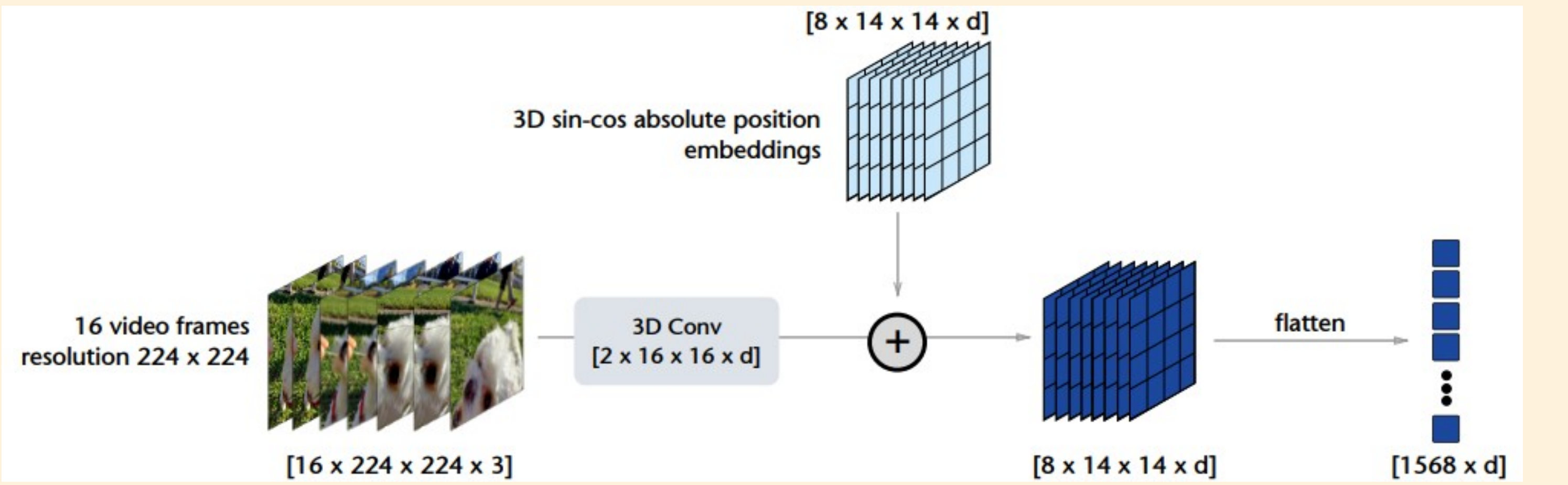
Source: Meta AI, V-JEPA 2 (2025), arxiv.org/abs/2506.09985.
A second, standard-pretraining worked example from the deck, at 256×256 resolution:
Tubelet size : (2, 16, 16)
Grid dims:
T' = 16 / 2 = 8
H' = 256/16 = 16
W' = 256/16 = 16
N_tokens = T' * H' * W' = 8 * 16 * 16 = 2048 tokens
Each tubelet passes through the Conv3d patch embedder and is projected to the encoder width (e.g., 1408 for ViT-g). The resulting token sequence is (2048, 1408).
EchoJEPA inherits this tubelet embedding unchanged from V-JEPA 2. Echocardiogram clips are tokenized with the exact same 3D convolution, just at echo's own resolution and frame rate.
3D RoPE
I-JEPA uses a fixed 2D sin-cos positional encoding, added once at the input and never touched by gradients. V-JEPA 2 replaces this with 3D Rotary Position Embeddings (RoPE), applied inside every attention layer rather than added once upfront. The extra axis encodes position along time (T), in addition to height (H) and width (W), so the model can tell "the same patch, a different frame" apart from "a different patch, the same frame".
EchoJEPA inherits 3D RoPE unchanged from V-JEPA 2. The same T/H/W structure applies directly to echo video clips, so no changes are needed here.
Masking and scaling in EchoJEPA
The masking mechanism itself, multiblock tube masking, holding the same spatial rectangle constant across every frame so the model must infer what happens inside it over time, is inherited unchanged from V-JEPA 2. What EchoJEPA does re-tune are the scale parameters, adapted to the physical constraints of an ultrasound fan:
- Context mask scale: 0.5–1.0 of the frame, wider than the default, to preserve enough visible anatomy inside a fan-shaped echo frame where much of the rectangular image is black background outside the sector
- Aspect ratio augmentation: 0.9–1.1, far narrower than I-JEPA's 0.75–1.5, respecting the fan's fixed geometry rather than sampling arbitrarily elongated crops
- Input resolution: 112×112 to 224×224, lower than V-JEPA 2's 256/384, since echo images are inherently lower-resolution than natural video
- Temporal resolution: 4–24 fps, variable per clip, since heart rate varies across patients, unlike V-JEPA 2's fixed fps
I-JEPA vs. V-JEPA 2 vs. EchoJEPA, axis by axis
The core algorithm doesn't change across these three. Every difference below is either a domain upgrade (image → video → cardiac video) or a scaling decision.
| Axis | I-JEPA | V-JEPA 2 | EchoJEPA |
|---|---|---|---|
| Modality | Static images | Natural videos | Echocardiogram videos |
| Patch unit | 2D patch, 16×16 | 3D tubelet, 2×16×16 | 3D tubelet, 2×16×16 |
| Token count (typical) | 256 (14×14 grid, 224px) | 2048 (8×16×16, 16-frame 256px) | Varies by fps / crop |
| Positional encoding | Fixed 2D sincos (no grad) | 3D RoPE per attention layer | 3D RoPE (inherited) |
| Encoder backbone | ViT-H/14, ~630M params | ViT-g/16, ~1B params | ViT-G 1.1B (EchoJEPA-G); ViT-L 300M (EchoJEPA-L) |
| Predictor | 12-layer ViT, 384-wide | 12-layer ViT, 384-wide (22M) | 12-layer ViT, 384-wide (inherited) |
| Loss | Smooth L1 | L1 | L1 |
| EMA momentum | Ramp 0.996 → 1.0 | Fixed (no ramp) | Fixed (inherited) |
| Masking | Multiblock 2D (spatial blocks) | Multiblock 3D (spatio-temporal tubes) | Multiblock 3D (inherited) |
| Context mask scale | 0.85–1.0 | Multiblock tubes | 0.5–1.0 (wider; preserves anatomy in a fan-shaped echo frame) |
| Aspect ratio aug | 0.75–1.5 | Standard | 0.9–1.1 (narrow; respects fan geometry) |
| Input resolution | 224×224 | 256×256 pretrain, 384×384 cooldown | 112×112–224×224 (echo is inherently low-res) |
| Temporal resolution | N/A | Fixed fps | 4–24 fps (heart rate varies across patients) |
| Training data | ImageNet, 1.28M images | VideoMix22M, ~22M videos | 18.1M echo clips (G) / 525K MIMIC-IV (L) |
| Downstream head | Linear / attentive probe | Probe-based eval | Multi-view attentive probe: 4 self-attention blocks, learnable view + clip embeddings, view dropout p=0.1 |
| Domain adaptations | None | None | Physics-informed perturbations: speckle, depth attenuation, fan geometry |
Table 6. The one conceptual addition V-JEPA 2 makes over I-JEPA: its tube masks hold the same spatial rectangle constant across every time step, forcing the model to infer what happens inside a region over time from the surrounding context, learning motion and dynamics, not just static appearance.
Why echocardiography breaks every existing foundation model
Ultrasound speckle is structured noise, not signal. It shows up as a grainy, seemingly random texture caused by constructive and destructive interference between the acoustic wavefront and tissue scatterers too small to resolve individually. Two frames of the exact same heart, captured a millisecond apart, show identical anatomy and completely different speckle. It's noise that regenerates itself every frame.
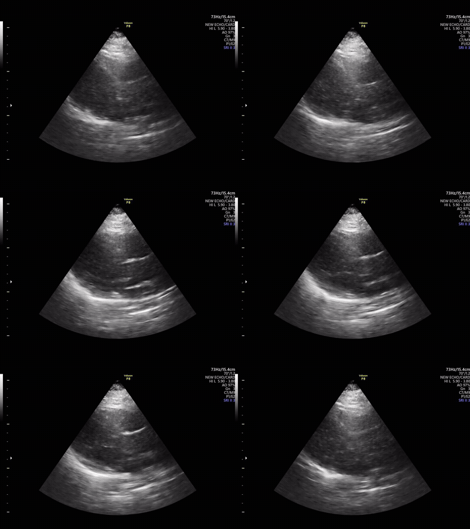
That single fact is enough to break most of the standard foundation-model recipes when they're pointed at echo:
| Problem | How it manifests |
|---|---|
| Speckle sensitivity | Pixel-reconstruction models (VideoMAE/MAE) must reproduce speckle faithfully; their representations encode acquisition texture, not anatomy. |
| Contrastive collapse | Text-supervised models (EchoPrime, PanEcho) rely on echo reports, which describe findings, not geometry; they learn semantic labels rather than structural representations. |
| Single-view bottleneck | Most models process one clip at a time: tasks like RVSP that require integrating measurements across views (Apical TR velocity + Subcostal IVC) cannot be computed from any single embedding. |
| Distribution shift | Models trained on adult anatomy fail on pediatric hearts (different size, heart rate, geometry) unless the representations encode transferable structure rather than population-specific statistics. |
Table 7. Why standard foundation-model recipes break when pointed at echocardiography.
EchoJEPA's answer
EchoJEPA applies the Joint-Embedding Predictive Architecture to echocardiography video. Instead of reconstructing pixels, it predicts the representation of masked spatiotemporal regions from visible context, entirely in latent space.
Why this solves the speckle problem: the EMA target encoder is updated slowly (an exponential moving average of the context encoder). Its representations are stable averages over many gradient steps; speckle, which is i.i.d. noise per frame, averages out. Anatomically stable structures (chamber walls, valve motion, geometry) are reinforced because they're consistent across time and views.
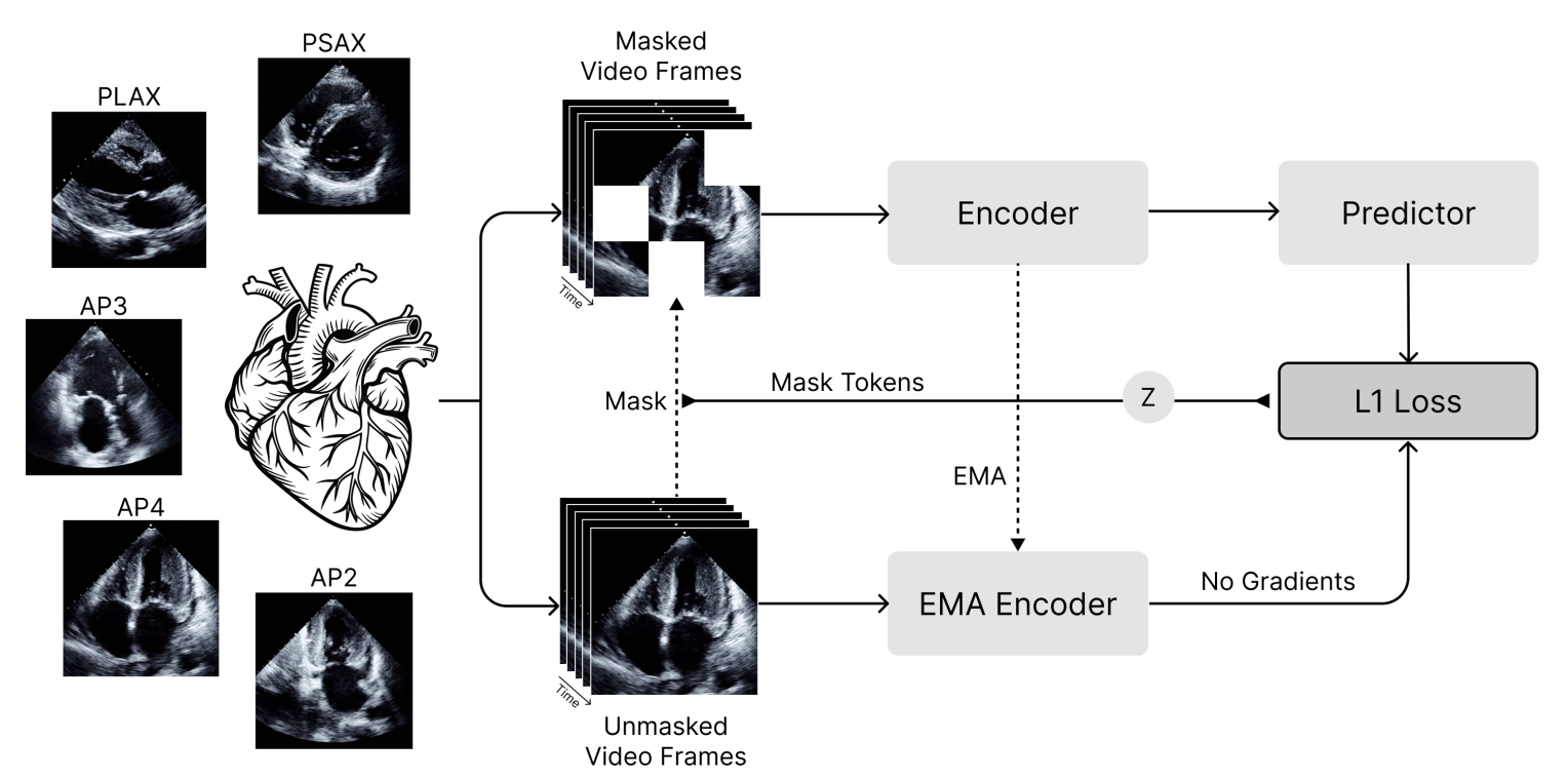
Source: EchoJEPA paper (2026), Fig. 1.
Contributions of the paper
- EchoJEPA. A foundation model using latent prediction pretrained on 18 million videos across 300K patients, the largest echocardiography corpus to date, achieving state-of-the-art performance on LVEF estimation and right ventricular systolic pressure (RVSP) prediction, demonstrating that latent prediction outperforms pixel reconstruction for ultrasound.
- Unified evaluation protocol. A standardized benchmark with frozen backbones, identical probes, and consistent hyperparameter search across all baseline models, enabling fair comparison of representation quality.
- Robustness benchmarks. Physics-informed perturbations using depth attenuation and acoustic shadow, revealing that EchoJEPA degrades 86% less than EchoPrime under acoustic perturbations.
- Public release. EchoJEPA-L, the first open-source JEPA-based echocardiography foundation model, trained on MIMIC-IV-Echo, is open-sourced alongside the evaluation framework at github.com/bowang-lab/EchoJEPA.
- Scale. EchoJEPA-G is pretrained on 18.1 million echocardiogram videos across 300,000 patients (the largest echo pretraining corpus assembled to date) behind a ViT-G encoder at 1.1B parameters. A smaller, publicly released variant, EchoJEPA-L, is pretrained on the 525K videos in MIMIC-IV-Echo.
- Multi-view probing framework. A method using factorized video stream embeddings and attention masking to integrate information across echocardiographic views without view-specific components. A single echocardiography study isn't one video; it's a collection of clips acquired from different transducer positions (Apical 4-chamber, Parasternal long/short axis, Subcostal, and more). The encoder processes each clip on its own, with no awareness that the others exist. A separate study-level attentive probe is what fuses them: it takes the per-clip embeddings from every acquired view and combines them with cross-attention into one study embedding.
Right ventricular systolic pressure is the clean test case for whether that fusion is doing real work, because it is structurally a two-view measurement:
RVSP = 4 × (TR jet velocity)² + RA pressure
└─ Apical view ──┘ └── Subcostal IVC ──┘
Why a standardized probe is required
This is the design choice that makes the benchmark fair: every model being compared (EchoJEPA, EchoPrime, PanEcho, VideoMAE) uses the same probe architecture, the same LR/weight-decay sweep grid, and the same multi-view fusion strategy. The only thing that differs is the frozen encoder producing the tokens; any difference in downstream performance is therefore a difference in what the encoder learned, not in how the probe was tuned.
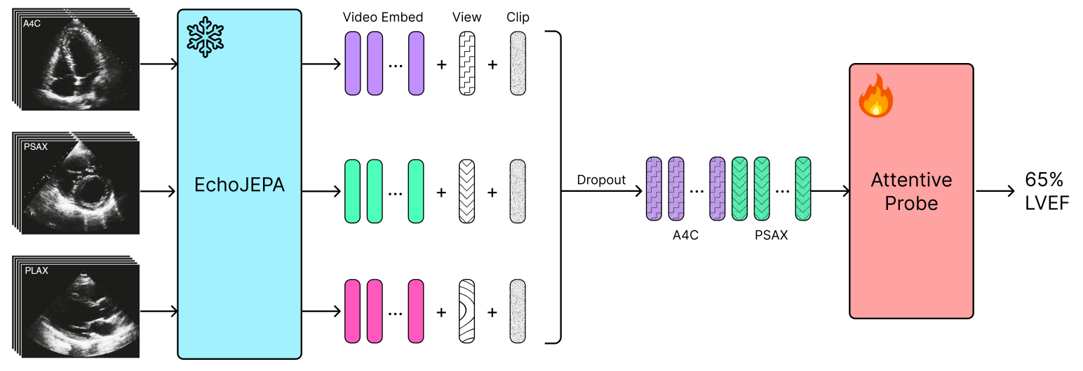
Source: EchoJEPA paper (2026), Fig. 2.
Any model that only ever probes one clip at a time is structurally incapable of getting this right, no matter how good its encoder is, which makes RVSP a useful way to tell "the encoder is strong" apart from "the whole system reasons correctly."
Architecture 3: Inside the multi-view attentive probe
- Input: Views & Clips
-
- A study is N views (Apical 4-chamber, Parasternal long/short axis, Subcostal, and more) × M clips per view; the default configuration is N = 9 views and M = 2 clips, giving 18 clips total
- Each clip is a 16-frame, 224×224 video, matching the tubelet embedder's expected input shape
[B, C=3, T=16, H=224, W=224]
- Frozen Encoder (f)
-
- This slot is whichever pretrained video encoder is being evaluated: EchoJEPA (ViT-G, 1.1B params, or the smaller ViT-L, 300M), or a baseline such as EchoPrime, PanEcho, or VideoMAE (EchoMAE) swapped in for comparison. It embeds each clip independently; it never sees the other clips or views at this stage
- A
Conv3d(2×16×16)tubelet embedder turns each 16-frame clip into a grid of 8×14×14 = 1568 tokens of width D (1408 for ViT-G) - No gradients flow into the encoder anywhere in this pipeline; only the probe sitting on top of it is trained
- Concatenate
-
- The per-clip token sequences from all 18 clips are concatenated along the sequence dimension into one long sequence: 18 × 1568 = 28,224 tokens
- Why early fusion: the probe can learn cross-view relationships, for example correlating the Apical view's LV size with the Parasternal view's wall thickness, because all tokens sit in the same attention context; a single-clip encoder never could
- Slot Embeddings
-
- The encoder gives all 18 slots identical-looking tokens; it has no way to know which view or clip each token came from. Slot embeddings inject that positional information by adding a learned vector of width D (1408 for ViT-G) to every token in a slot
- Two small learned embedding tables fix that:
view_embed: 9 entries, keyed byview_id = slot_id // clips_per_view
clip_embed: 2 entries, keyed byclip_id = slot_id % clips_per_view
Both are broadcast to all 1568 tokens in a slot via
slot_emb.repeat_interleave(Nslot=1568, dim=1)
and added elementwise (⊕) - Why factorized: decouples the 9-dimensional view axis from the 2-dimensional clip axis. Without factorization you'd need 18 independent embeddings and lose generalization across different orderings
- During training only, entire views are randomly dropped with probability 0.10, so the probe learns to be robust to whatever subset of views a real study happens to include
- Self-Attention Blocks
-
- Three standard pre-norm transformer blocks mix information across all 28,224 tokens, regardless of which view or clip they came from, each a residual connection:
x = x + MHSA(LayerNorm(x))
x = x + MLP(LayerNorm(x)) - MHSA:
head dim = D / num_heads = 1408 / 16 = 88
Q, K, V each projected:
[B, 28224, 1408] → [B, 16, 28224, 88]
Attention matrix:
[B, 16, 28224, 28224] - MLP:
hidden_dim = D × mlp_ratio = 1408 × 4.0 = 5632
Linear(1408→5632) → GELU → Linear(5632→1408) - This is where cross-view reasoning actually happens: a token from the Apical view can attend directly to a token from the Subcostal view
- Three standard pre-norm transformer blocks mix information across all 28,224 tokens, regardless of which view or clip they came from, each a residual connection:
- Cross-Attention (Pool)
-
- A single learned query token:
self.query_tokens = nn.Parameter(torch.zeros(B, 1, 1408))
trunc_normal-initialized, is the only query; the full 28,224-token sequence serves as keys and values - The CrossAttentionBlock uses the query token as Q and the full 28,224-token sequence as K/V:
Q: [B, 1, 1408]K/V: [B, 28224, 1408] - Attention:
softmax(Q·Kᵀ/√88)·V, i.e.[B, 1, 28224] × [B, 28224, 1408] → [B, 1, 1408]
collapsing the entire study, every view and every clip, into one vector - After the MLP, squeezing the singleton dimension gives the final
[B, 1408]study embedding: this is the pooling step that turns "many clips" into "one study"
- A single learned query token:
- Linear Head
-
- Regression (LVEF, RVSP):
self.regressor = nn.Linear(D, num_targets, bias=True)
mapping[B, 1408] → [B, 1], e.g. LVEF in % - Classification (13-class view, per codebase config):
self.linear = nn.Linear(D, num_classes, bias=True)
mapping[B, 1408] → [B, 13] - The head architecture is swapped per task, and each task is trained separately with its own head; the frozen encoder and the rest of the probe (concatenation, slot embeddings, self-attention, cross-attention) share the same design across all three tasks, but are not one shared set of trained weights
- Regression (LVEF, RVSP):
Learning targets for the probe
Three tasks, each defined by a separate config. The probe head (a linear layer) is swapped per task; the 4-block transformer body is shared in design but trained separately for each.
Target 1: LVEF (Left Ventricular Ejection Fraction)
LVEF is a single-view task; the Apical 4-chamber view captures both the LV inflow tract and outflow tract, giving enough geometry. No cross-view reasoning is needed; the probe runs single-view, not multi-view.
Target 2: RVSP (Right Ventricular Systolic Pressure)
RVSP only uses 4 clips from 2 views:
└─ from Apical ─┘ └── from Subcostal ──┘
TR velocity is the tricuspid regurgitation jet velocity (m/s), measured in the Apical view via continuous-wave Doppler. RAP is right atrial pressure (mmHg), estimated from IVC diameter and collapsibility measured in the Subcostal view. RVSP is the litmus test for whether multi-view reasoning actually works; competitors that use single-view probes cannot compute it correctly regardless of encoder quality.
Target 3: View Classification (13 classes)
Probe output is a [B, 13] softmax over view classes, trained with cross-entropy loss. This is a per-clip task, not a study-level aggregation.
Note: each of the three tasks is trained and probed independently.
Datasets used
| Dataset | Type | Size | Used for |
|---|---|---|---|
| Toronto (internal) | Proprietary, multi-view | 150,000 studies | Probe training + internal validation |
| Chicago (internal) | Proprietary, multi-view | 60,000 studies | External holdout site (out-of-distribution) |
| EchoNet-Dynamic (Stanford) | Public, single-view (A4C) | 10,030 videos | LVEF cross-site evaluation; adult source for pediatric transfer |
| EchoNet-Pediatric | Public, single-view | 3,516 videos | Zero-shot pediatric generalization target |
| MIMIC-IV-Echo | Public, multi-view | 525,000 videos | EchoJEPA-L pretraining |
| Proprietary (UHN) | Proprietary, multi-view | 18.1M videos, 300K patients | EchoJEPA-G pretraining |
Table 8. Datasets used across EchoJEPA pretraining and evaluation.
Architectures
EchoJEPA trains two variants at different scale, EchoJEPA-G and EchoJEPA-L; the weights for EchoJEPA-L are open-sourced.
| Component | EchoJEPA-G | EchoJEPA-L |
|---|---|---|
| Encoder backbone | ViT-G/16, 1.1B params, 40 layers, width 1408, 16 heads | ViT-L/16, 300M params, 24 layers, width 1024, 16 heads |
| Tubelet embedder | Conv3d(3, 1408, kernel=2×16×16, stride=2×16×16) | Conv3d(3, 1024, kernel=2×16×16, stride=2×16×16) |
| Positional encoding | 3D RoPE (T/H/W axes, applied per attention layer) | 3D RoPE |
| Predictor | 22M, 12 layers, width 384 | 22M, 12 layers, width 384 |
| Pretraining loss | L1 in latent space (masked target regions only) | L1 in latent space |
| Target encoder | EMA of context encoder, fixed momentum | EMA of context encoder |
| Pretraining data | 18.1M proprietary echo videos | 525K MIMIC-IV-Echo |
| Attentive probe | depth=4, 16 heads, D=1408 | depth=4, 16 heads, D=1024 |
Table 9. EchoJEPA-G and EchoJEPA-L component specifications.
Results: EchoJEPA vs. Competing Methods
All models are evaluated with identical probes: same architecture (depth=4, 16 heads), same LR/weight-decay sweep, same multi-view fusion. The only variable is the frozen encoder.
- EchoPrime. Contrastive VLM, trained on 1M+ echo videos with report supervision.
- PanEcho. Contrastive model trained on 1M+ echo-report pairs.
- EchoMAE-L. Pixel reconstruction (VideoMAE objective), same ViT-L backbone as EchoJEPA-L; the direct apples-to-apples ablation of latent vs. pixel prediction.
- EchoJEPA-L. V-JEPA 2 latent prediction, ViT-L, trained on 525K public MIMIC-IV-Echo videos.
- EchoJEPA-G. V-JEPA 2 latent prediction, ViT-G (1.1B), trained on 18.1M proprietary echo videos.
Summary
| Task | Metric | EchoMAE-L | EchoPrime | EchoJEPA-G | vs. EchoMAE-L | vs. EchoPrime |
|---|---|---|---|---|---|---|
| LVEF (Stanford) | MAE ↓ | 8.52 | 4.87 | 3.97 | −53% | −19% |
| View ID (1% labels) | Acc % ↑ | 21.8 | 21.6 | 78.6 | +260% | +264% |
| RVSP (Toronto) | MAE ↓ | 5.36 | 5.65 | 4.54 | −15% | −20% |
| Robustness | Avg. degradation | +0.5%† | +16.8% | +2.3% | n/a | −86% |
| Pediatric zero-shot | MAE ↓ | 6.79 | 5.10 | 4.32 | −36% | −15% |
Table 10. The headline numbers across every task: latent prediction (EchoJEPA-G) beats both the pixel-reconstruction baseline (EchoMAE-L) and the strongest contrastive/text-supervised baseline (EchoPrime) on accuracy, label efficiency, robustness, and cross-population generalization at once.
Attention visualization
Decoding what each model's encoder actually attends to, before and after finetuning on echocardiograms, shows why latent prediction produces more anatomically grounded representations.
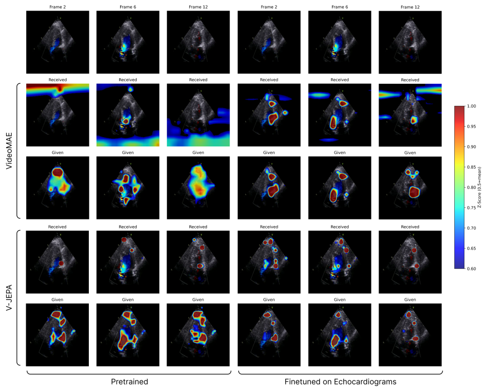
Source: EchoJEPA paper (2026), Fig. 4.
Latent space analysis
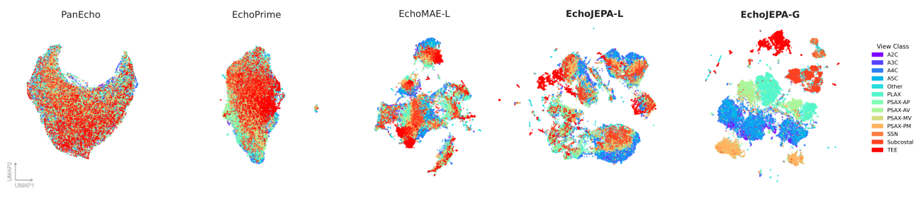
Source: EchoJEPA paper (2026), Fig. 5.
What this means going forward
In November 2025, LeCun announced his departure from Meta after twelve years (five as FAIR's founding director, seven as Chief AI Scientist) to co-found Advanced Machine Intelligence Labs (AMI Labs) in Paris. AMI Labs targets industrial, robotic, and healthcare applications using JEPA-based learning from video and sensor data; the fundraise signals investor confidence that world models (not LLM-style next-token prediction) are the path forward.
The JEPA family has fanned out quickly since. LLM-JEPA applies the objective to language, predicting latent token-sequence representations instead of the next token, and outperforms standard LLM training objectives. LeJEPA is a leaner, theoretically grounded reformulation of the whole framework that removes ad-hoc heuristics. ACT-JEPA conditions on actions for efficient policy representation learning in robotics. LeWorldModel adds value shaping to the JEPA world model's representation space to enable planning. VL-JEPA predicts continuous text embeddings for vision-language tasks instead of generating tokens autoregressively. US-JEPA generalizes the approach to ultrasound imaging in general, learning anatomical dependencies and tissue-texture relationships across multiple ultrasound modalities. And V-JEPA 2.1 pushes denser spatiotemporal features out of the original video model, setting new marks on Ego4D and EPIC-KITCHENS.
The JEPA family, as of this writing
| Paper | arXiv | Date | What it does |
|---|---|---|---|
| LLM-JEPA | 2509.14252 | Oct 2025 | JEPA objective for LLMs: predicts latent representations of token sequences rather than tokens themselves; outperforms standard LLM training objectives |
| LeJEPA | 2511.08544 | Nov 2025 | "Lean JEPA", a theoretically grounded reformulation removing ad-hoc heuristics; scalable and clean |
| ACT-JEPA | 2501.14622 | Jan 2026 | Action-conditioned JEPA for efficient policy representation learning in robotics |
| LeWorldModel | 2601.00844 | Dec 2025 | Adds value shaping to the JEPA world model's representation space to enable planning |
| VL-JEPA | 2512.10942 | Feb 2026 | Vision-language model predicting continuous text embeddings instead of autoregressive token generation: 50% fewer trainable parameters, 2.85× fewer operations at inference via selective decoding |
| US-JEPA | 2602.19322 | Feb 2026 | JEPA applied to general ultrasound imaging: learns anatomical dependencies and tissue-texture relationships across multiple ultrasound modalities |
| V-JEPA 2.1 | 2603.14482 | Mar 2026 | Unlocks denser spatiotemporal features from V-JEPA 2: state of the art on Ego4D (7.71 mAP) and EPIC-KITCHENS (40.8 Recall@5) |
Table 11. The JEPA family tree, as of this writing.
Sources
- Yann LeCun's Joint Embedding Predictive Architecture (JEPA) and the General Theory of Intelligence
- LeCun, A Path Towards Autonomous Machine Intelligence (2022), openreview.net/pdf?id=BZ5a1r-kVsf
- I-JEPA: The first AI model based on Yann LeCun's vision for more human-like AI
- Assran et al., I-JEPA: Self-Supervised Learning from Images with a Joint-Embedding Predictive Architecture (2023), arxiv.org/abs/2301.08243
- MC-JEPA: A Joint-Embedding Predictive Architecture for Self-Supervised Learning of Motion and Content Features (2023), arxiv.org/abs/2307.12698
- Bardes et al., V-JEPA: Revisiting Feature Prediction for Learning Visual Representations from Video (2024), arxiv.org/abs/2404.08471
- Garrido, Ballas, Assran et al., Intuitive physics understanding emerges from self-supervised pretraining on natural videos (2025), arxiv.org/abs/2502.11831
- Meta AI, V-JEPA 2 (2025), arxiv.org/abs/2506.09985
- EchoJEPA
- EchoJEPA codebase
- EchoJEPA paper
- x.com/aakashgupta/status/2046371351016161745